Introduction
This post aims to present a tool that can be used by students in the area of Control Systems. The tool consists in a virtual laboratory that simulates several dynamical systems. The tool is a WebApp implemented 100% in Javascript (the simulator) and can be easily accessed at:
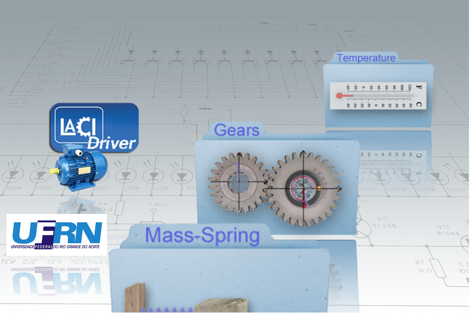
When you access the app, you will see a menu with “folders” that can be slided left or right. Each folder links to a simulation for a different system. Slide left or right to access the system and click on it to go to the simulation screen. The following figure shows the menu.
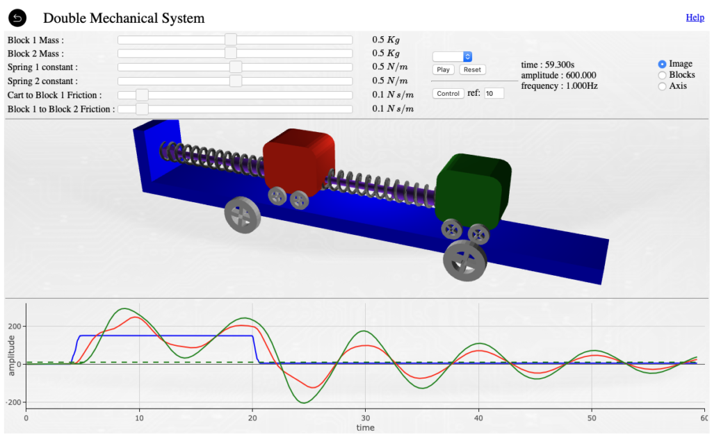
Each simulation runs in a standard interface that have controls to change the system’s parameters, control the flow of the simulation, see plots, etc. The next figure gives an example of such interface.
In the app, you can click on the Help link to obtain detailed information about the controls and objects in the interface.
To run the simulation, you just have to click on the “play” button. You will see immediately the time starting to increment and the plot region starting to show the values of the dynamical variables involved. Every system have one variable that you can control (input) and one or more outputs that follows the dynamics of the system that is being simulated. To apply an input, you can drag the mouse horizontally in the “canvas” region (middle part of the screen where the system is being animated). The blue plot bellow will show you the value of the input as you change it. As you change the input, the system responds in real time according to the input value.
Another way to apply an input to the system is via the “input” box. You can choose different types of inputs such as step, sinusoids, noise and etc. The parameters for those inputs are also controlled by dragging the mouse in the canvas area. This time, dragging horizontally changes the “frequency” of the input and dragging vertically changes its amplitude.
For each system, there are levels of “displays” in the canvas area. Some systems have an “axis” level where you just see arrows in the position corresponding to the associated values (input or output). That is useful when you want to check for precise values, errors and what not. Another possible display type is the “image” display. There, you will see a 3D representation of the system or a real picture depicting its state or behaviour. In the 3D visualisation, you can use the mouse wheel to rotate and tilt the camera. You can also press shift to zoom in or out.
External Controller
The app have a built in WebSocket server that “serves” the dynamic behaviour of each system to an external controller. It implements a simple ascii protocol that answers to commands allowing the client to read outputs and to apply something as input. This protocol runs continually as long as the simulation is being played. Because of that, it allows the implementation of closed loops systems with an external controller.
The protocol expects to read and write ascii values for the output, reference and input signals. The available commands are:
- get reference : Client should send this command to receive the current reference value from the simulator
- get outputs : Client should send this command to receive the current outputs from the simulator in a comma separated format.
- send input|xxxx : Client should send this command to apply value xxxx as input to the simulator.
By sending those commands in sequence, we can close the loop by implementing an external app that connects to the WebSocket and repeatedly keeps asking for output/reference, computes the control signal and sends it back as input to the system.
There is a python module that you can download here that implements this loop and instantiates a controller class that you can overwrite to implement your own control law.
Technically, the external controller is implemented as a WebSocket server (nor client) and the simulator acts as a client that can answer to commands coming from that server. This is absolutely transparent to the user. The only important technical aspect worth mentioning is that, due to security issues with WebSockets in modern browsers, you are allowed to use this feature only locally (within the same machine). That means that, if you want to implement your own server, you will be able to accept connections only from localhost clients.
Python module
The python module is very simple. It consists of two classes: Control and RemoteControl. The RemoteControl class is responsible for implementing the WebSocket interface and the main loop while the Control class implements the control logic. The RemoteControl receives an instance of the Control class with the implemented control logic and organises the calling of its methods in an infinite loop. After instantiating the RemoteControl class, you just need to call the method run() to start the server and be ready to serve as a controller.
The whole code for an external controller can be as small as the following code:
from ControlLib import *

controller = Control()
rc = RemoteControl(controller)
rc.run()
The loop implemented by the RemoteControl class consists in a simple sequence of commands:
- 1 – get reference value from simulator
- 2 – get output value from simulator
- 3 – compute the error
- 4 – compute the control signal
- 5 – send the control signal to the simulator
- 6 – go back to 1 and repeat
The default behaviour for the Control class is to output always zero. Hence, if you run the code showed above you will be disappointed 😅. In order to have something useful, you have to implement your own control class inheriting from Control and overwriting the method control().
The minimum useful control implementation can be something like:
from ControlLib import *

class MyControllerName(Control):

    def control(self):
        """
        Return the control signal.
        You can access the error at instant 0, -1, and -2 as:
        self.e(0), self.e(-1) and self.e(-2) respectively

        Obs.: To access more errors, create your controller with the
        command:
        controller = MyControllerName(T, n)
        where T is the sampling time (normally 0.3) and n is the order
        of the controller (how many errors you can access)
        For instance:

        controller = MyControllerName(0.5, 6)

        Will use a controller with 0.5s sampling time and will access
        from self.e(0) up to self.e(-5)
        """

        # in this simple controller, it applies a control signal that
        # is 90% the current error

        u0 = 3.1*self.e(0)

        return u0


controller = MyControllerName(0.2,3)
rc = RemoteControl(controller)
rc.run()
Now the server is already capable of doing something. In that case, a simple “proportional” P controller is implemented. There are two new and important aspects on this new example code. The first one is the fact that we have our own control class now (called MyControllerName in the example) and that class is being instantiated with two arguments. Those arguments are the sampling time and the controller order.
The sampling time is going to define how often the loop will read/write values to the simulator. This is exactly the role of sampling period in digital control. The second one is the controller order. It defines how many past errors the controller is able to provide. The default value of 3 means that we have access to the error at the instants 0 to -2 ![e[0]](https://www.dev-mind.blog/wp-content/ql-cache/quicklatex.com-3e0c81e14fb53e112c68830f5497d5b4_l3.png "Rendered by QuickLaTeX.com") ,
, ![e[-1]](https://www.dev-mind.blog/wp-content/ql-cache/quicklatex.com-c5199c2532645f5a27e56b07fe15ad0f_l3.png "Rendered by QuickLaTeX.com") and
and ![e[-2]](https://www.dev-mind.blog/wp-content/ql-cache/quicklatex.com-922101d9a09867502db0125aa84cb10a_l3.png "Rendered by QuickLaTeX.com") .
.
The second important aspect is how we read the variables to implement the controller. The Control class implements 4 basic methods: self.u(n), self.r(n), self.y(n) and self.e(n). They can be called to access the control signal, reference signal, output and error respectively. So, inside the control() method, we can call, for instance, self.e(-4) to access ![e[-4]](https://www.dev-mind.blog/wp-content/ql-cache/quicklatex.com-7261016e8cc65ab4a9cfc027691faf64_l3.png "Rendered by QuickLaTeX.com") (the error 4 instants in the past). Remember that to do that, you need to set the order to at least 5 in the second parameter of the control constructor (in our example, it would be something like control = MyControlName(0.3, 5)).
(the error 4 instants in the past). Remember that to do that, you need to set the order to at least 5 in the second parameter of the control constructor (in our example, it would be something like control = MyControlName(0.3, 5)).
Moreover, you can implement fancier controllers that have adjustable parameters, adaptive output, etc. You can override the constructor in the Control class and receive parameters that defines your controller (like gains, scales, etc). Since the RemoteControl class is only using the result of the control() method, you can have very sophisticated stuff implemented as long as, in the end, you return a single value. You can even have loops and entire algorithms implemented inside the control() method. You just have to make sure that it respects the sampling time and don’t freeze the execution for more than T seconds.
In summary, to use the system with an external controller, you:
- 1 – download the ControlLib module (from here) end save it in your computer (for instance at /home/user/webControl)
- 2 – Go to the folder, open a text editor and create your controller. Write your code like the example above and save it (for instance /home/user/webControl/mycontroller.py).
-
3 – Execute your controller. (for example, you can open a terminal and type the following command line)
$ python3 mycontroller.py
- 4 – Open the browser and access the app at www.dev-mind.blog/apps/control_systems/iDynamic/
- 5 – Choose a system, click “play” and then click “control”.
Thats it. The following video shows the system being used. As always, code is at GitHub. Feel free to clone, modify, rewrite, etc %-)

|
Demo Video 1 Demo Video 2 |
Muito bacana essa ferramenta, parabéns pela aplicação.
Valeu Caio! Muito obrigado!
Boa noite, estou utilizando esta aplicação na disciplina de Projeto de Sistemas de Controle – UFAL ministrada pelo professor Ícaro, para isso contruímos uma interface gráfica local que deve obter os sinais de saída apresentados nos experimento e mostrar tais sinais a interface gráfica. Além disso podemos escolher o sinal de entrada que será utilizado nesta aplicação web. Assim , como posso obter os sinais de saída mostrados no gráfico do IDynamic e plotar tais gráficos localmente? Obrigado!
Ola André,
Para obter os sinais, voce pode usar o exemplo em python the tem disponível no link do GitHub (no artigo tem o link no final). Basicamente os arquivos são um exemplo de um controlador. Como voce só quer plotar os gráficos, ignore a parte do código que calcula o sinal de controle e use apenas os valores de saída que o programa recebe. Ai voce pode criar seu próprio programa pra armazenar estes valores e ir fazendo um gráfico.
Ótimo, muito obrigado pela dica!
Opa, estou usando o projeto na disciplina de Projeto de Sistemas de Controle – UFAL ministrada pelo professor Ícaro. Porém, a comunicação é implementada utilizando websockets, que por sua vez utilizam o módulo asyncio. Dificultando muito trabalhar com threads e desenvolver interfaces gráficas. Tentei efetuar a comunicação utilizando um servidor socket comum, mas o simulador não retorna os dados corretos e encerra a conexão em seguida. Há como prover um exemplo de servidor websocket que funcione com threads, ou um servidor socket que seja compatível com o simulador?
Ola João,
Realmente o async io não gosta muito de rodar junto com Threads… Tem algumas soluções… Uma delas é tentar escrever as funções de plot também asynchronas e ver se da pra não interferir no tempo de amostragem do controlador. Outra é usar IPC (inter process comunication) pra mandar os dados que voce quer plotar para outro script (ou processo) que plota os gráficos.
Vamos tentar marcar com Icaro e quem tiver interessado pra tentarmos ver qual solução fica mais fácil.