Introduction
This post is the continuation of a previous post about making an AO system simulation using blender (+friends). In this post we will talk about the implementation of the simulator. For details about what we simulate, please refer to the previous post. As always, everything is on GitHub.
In summary, we use blender together with python, Matlab and a bit of (OSL) Open Shading Language to simulate a simple (although quite didactic) AO system. We simulate the star light, the medium where the light passes through (atmosphere), the wavefront sensor that measures the phase deformation and the deformable mirror that corrects for that deformation. We also compute all the cool math that are used in a real AO system with the data generated by our simulator. It is important to mention that this is real simulator not an emulator. That means that we really simulate the physics of the light diffracting and reflecting off of surfaces. We could “emulate” an AO system by having a pre-computed interaction matrix for some pre-defined objects and show how SPFs, Dm commands, etc would behave. However, that’s not the case. We really simulate the light and compute interaction matrices, DM commands, etc all using “real” raytraced light data.
The whole simulator is a little bit intricate because a lot of problems had to be solved in order to make it possible. To better explain the whole process, the next figure illustrate the “usage” of the system. And the vídeo shows the system in action. Later on we progressively explain how things work internally and how they were done.
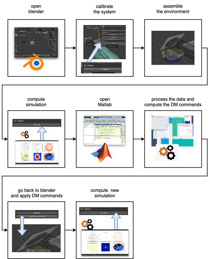
Figure 1: Simulator usage
Figure 2: System in action (better viewed in fullscreen)
In the system, we have a simulated point source of light, a deformable mirror and a wavefront sensor. Each one is made up using normal blender objects carefully adapted or picked to work like its real counterpart (to simulate, not emulate).
When we open the blender file, you have all the components of the simulator. In summary, there are several “parts” that constitutes the blender side of the simulator itself:
- 3D model of the physical parts
- Light source
- Wavefront sensor
- Deformable mirror
- Some translucent objects to be used as medium where the light passes through
- Lenses
- Atmosphere
- Special material to be used as detector
- detector.osl
- Python code for panel, and classes
- panel.py
- WFS.py
- DM.py
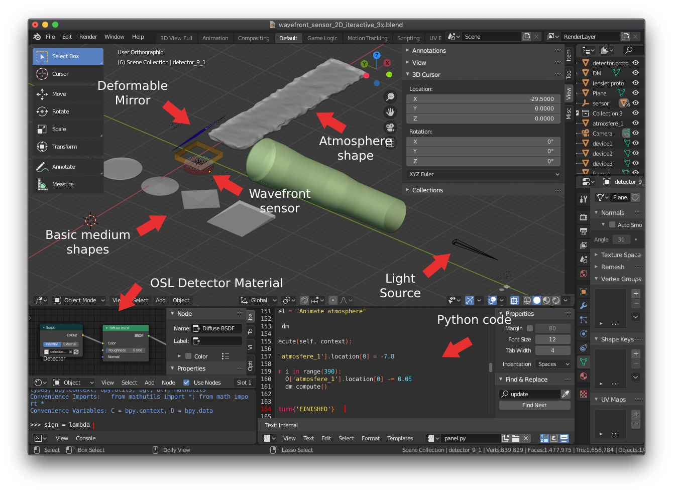
Figure 3: Blender components
The system itself, as said in the beginning, is composed by several scripts in Python and Matlab. The system started as a small experiment to learn about AO. Because of that, several parts “grew” in functionality while others remained as they were. In the end, the system itself is kind of a “Frankenstein”, mixing Inter-Process communication with file bases information exchange, among other “gambiarras” (Portuguese word for “informal technical adaptation” 😅). The overview of the technologies and parts involved in the implementation are shown in the following figure. In the future, if time allows, I’ll try to have one big python script to control everything and avoid this “soup” of scripts going back and forth with information.
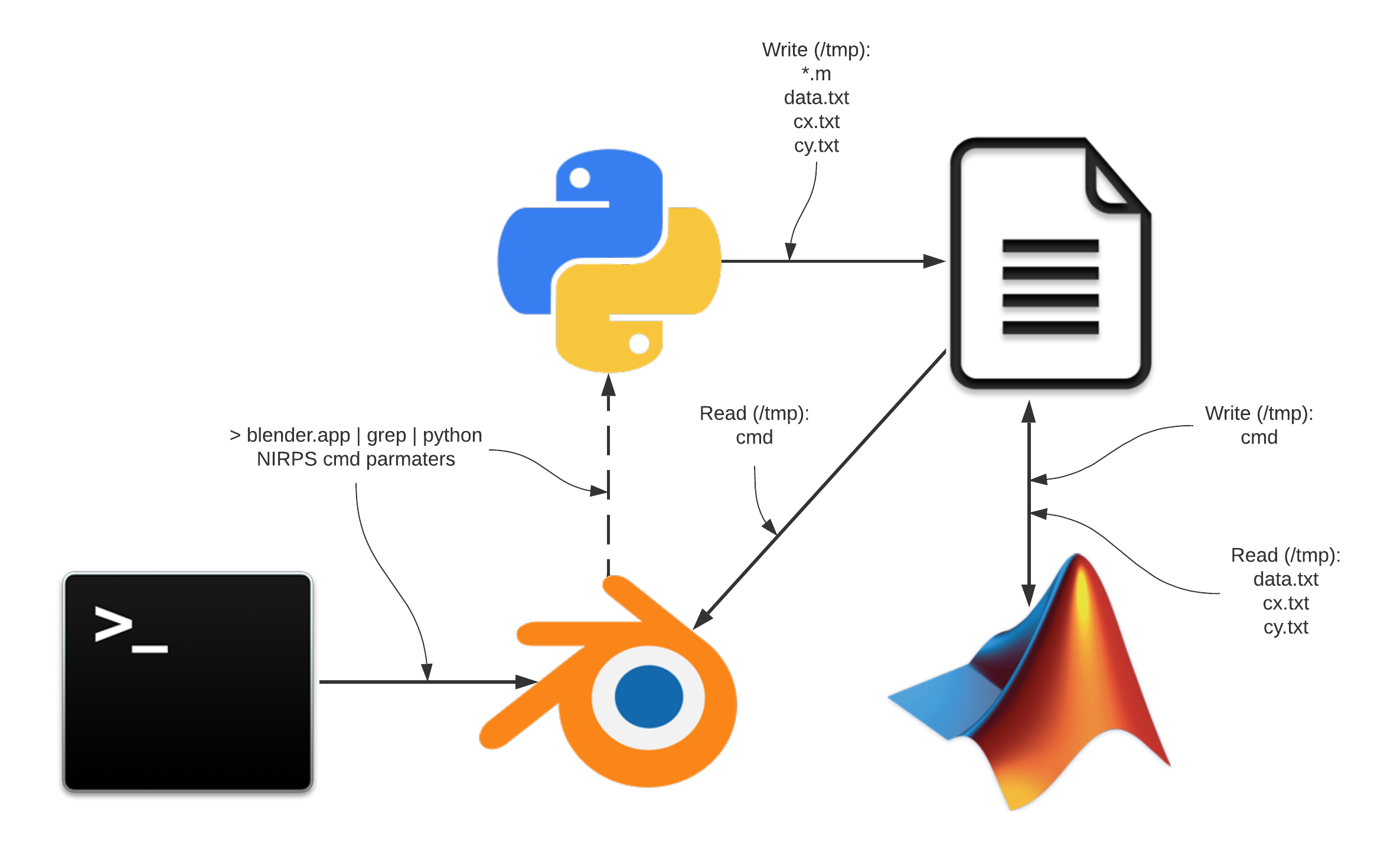
Figure 4: Diagram of the system indicating its components
Blender is the center of everything. It communicates with a python script via IPC using a terminal piping system (explain why later) called PipingServer. Another python script inside blender sends commands to this PipingServer in order to, for instance, plot some measurement or save data. This PipingServer have commands to save the data as Matlab files that later on will be used to communicate with a Matlab script that will compute the AO Business (interaction matrix, command matrix, etc…). Matlab then saves data that will later on be read back by blender to use in the deformable mirror.
Referring back to the first figure, we will now go a bit further in details about the sequence that the user must follow to use the system.
- Open blender: In order to allow blender to interact with the external script, we open it using a unix piping scheme. This will create a stdin connection between blender and the PipingServer.
- Calibrate the system: We run the panel.py script inside the blender file to execute the GUI part of the system. There, there are several buttons to control the AO system. The first thing we should do is to mark “calibrate” check box and click “compute”.
- assemble environment: The user now can place any object in the light path. There is a small square close to the WSF and the DM where the user can put, say, a lens or any transparent object.
- Compute simulation: Once the system is calibrated, we can start to use it. Now, the button “compute” will tell the system to take a snapshot of the “star” and plot (in the external python window) the data related to the measurement. It will plots things like WSF “image”, PSF, slopes, etc. Anything in the light path will “distort” the light, generating a pattern of wavefront phase in the WFS. Next, the user can use the external plot window to see the PSF and even to have a simulated image of how this element in the light path is distorting images that are far away form the system (see NIRPS Logo in the next figures).
- Open Matlab: Once a measurement is done, data will be automatically be saved and some Matlab files are going to be placed in the /tmp folder. In Matlab, there will be a script that will read those Matlab files and process them.
- Process the data in Matlab: When the user runs the Matlab script, it will gather the data produced by the measurement done in blender and compute all the AO business. It assembled an interaction matrix, apply it to the recently read slopes and generates a DM command vector. Everything is illustrated by tons of plots describing the process and the data used. Matlab then saves the commands as a text file in the /tmp folder.
- Go back to blender and read the DM commands: Now that Matlab computed the DM commands, the user loads them by clicking “Load DM commands” button. This will tell blender to read the saved text file and literally deforms the DM element with the shape computed by Matlab.
- Compute new simulation:
- Appreciate the result: Everything that happens is completely physically simulated (see raytrace part later). There is no pre-defined shape related to a pre-defined set of slopes or deformations of the mirror. ANYTHING translucent that we put in the light path will realistically refract the rays and that refraction will be measured in the WSF component. Also, deforming the mirror will reflect the ray to another direction that also will be captured by the WFS. Hence, when Matlab compute the mirror commands, its computing the exact shape that deforms the rays in the exact way so as to undo whatever deformation happened by the refractions caused by the object put in the light path. Moreover, since we are in a 3D modelling software, one can put ANY shape in the light path and correct for it as long as its in the range of the WSF. I cannot think a better way to learn and get a sense of the subject of adaptive optics!
With the mirror deformed, we can click again in the “compute” button (keeping the object in the light path). The result is, if everything goes well, an “undeformed” image in the plots.
The system
This simulator is far from being a product. There are professional simulators available that can be used professionally. However, as a leaning tool, it has being proven (at least to me) very useful. The official and professional softwares uses a technique called raytrace to simulate the light and do all this magic that I just described. The central point is very very simple: Shoot a “ray of light” at an angle  from a source in the direction of a WFS and measure its arriving angle. If it is the same , there is no phase shift in the light. That means that there was no refraction in the path of ray (or there was some that was corrected). Although this is a very simple principle, it is very very powerful when we apply to millions of light rays.
So, to perform all this “mathemagic” of AO simulation, we would need to implement a raytrace. Although it would be a small one, we would need to deal with all the 3D business of line interceptions, 3D shaped object representation, material refraction computations, etc, etc, etc. In this project we exploited one of my favorite software: blender. Blender is a 3D rendering software and it has a very powerful raytracer called Cycles. Moreover, it is monstrously customisable via python internal API. Basically, all the functions that we do manually in the software have an exposed python command that can be called via script internally in blender. It is possible even to implement GUI with buttons, panels. etc.
Using this internal python API, we can make a panel for the user to interact with. Buttons like “Compute”, “Load DM commands”, etc. Together with that, we can use the whole 3D apparatus to build the environment. We can put a mirror, make lenses, etc. When I say “make lenses” I don’t mean to code the math of light refraction based on the internal radius and bla bla bla. I mean literally “make a lens”. Place two goals spheres with some intersection and ask blender to subtract one form the other. Thats it. its really really a “mechanical” process. All the business of refraction, angles, radius, etc, etc will be dealt with by the raytracer! This is exactly what you will find in the blender file used in this simulator. Coming back to figure 3, you will see exactly that. The next figure illustrates the idea for better understanding:
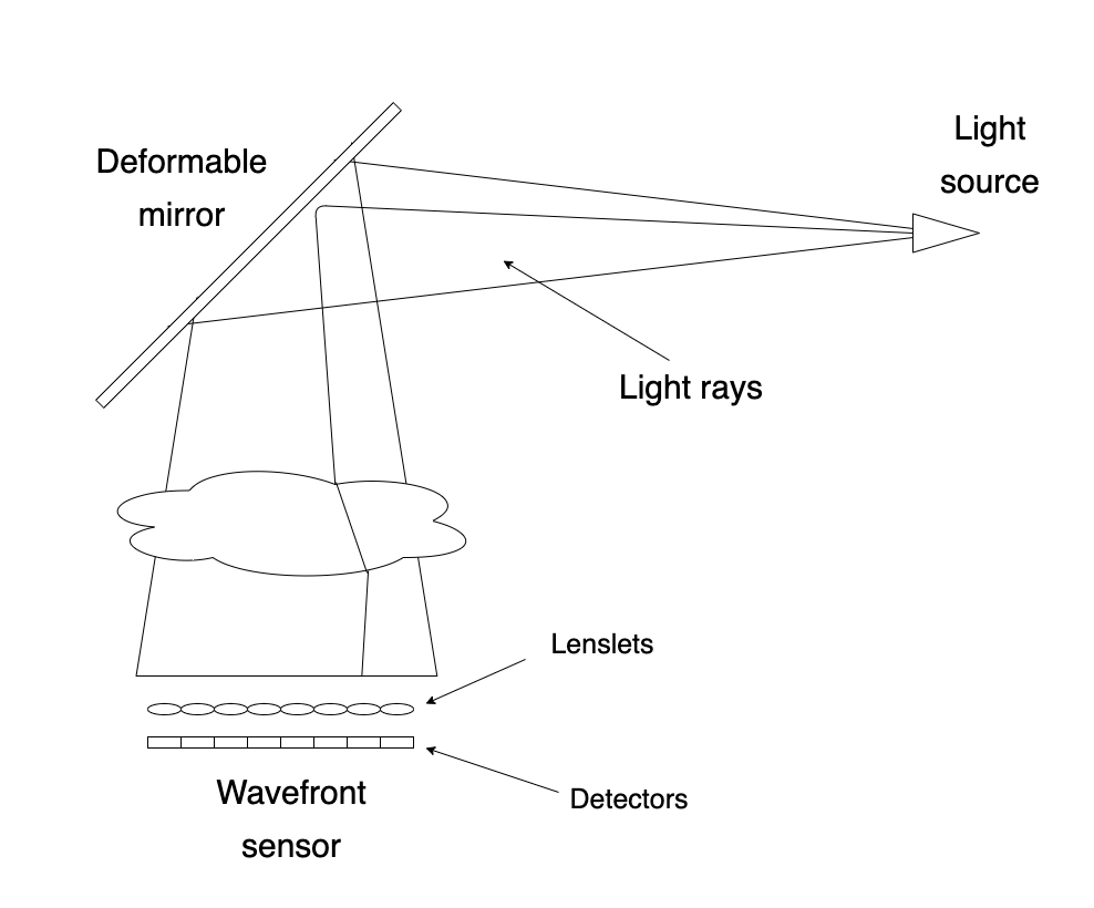
Figure 5: Raytrace diagram used in the blender file
As you see in the figure, we have a source of rays (triangle in the right) that shoots rays against the mirror (tilted square in the left). The rays reflect down and passes through the medium (translucent object). The medium refracts the light ray before reaching the WFS. The WFS it very tricky to implement but is basically composed by a set of micro lenses (lenslets I think is the technical name) and a set of detectors.
Now, in summary, when we press the “Compute” button, blender generates tens of thousands of light rays using Cycles. Each one finds its way to the detector reflecting off of the deformable mirror and refracting when passing through the medium object. The micro lenses (which are also regular objects made in blender) focus the light in the center of the detectors in order to simulate the behaviour of the WFS. The light that arrives in the detector is somehow processed and sent to Matlab that uses it to compute the exact deformation needed to be applied at the mirror and undo the refractions that the light suffered when passed through the medium. Then, the user loads the commands which literally deforms the mirror, performing the correction.
The challenges involved
Up to this point, I assume you understood what the simulation is doing. Now is time to know how it does it. As stated before, a lot of “tricks” had to be thought out in order to overcome all the challenges. In the following sections we will detail each one.
Artificial Star
The first trick was to get blender to do the raytrace job for us. Normally we would think of placing a light source as the simulated “star” so that “rays of light” will go from the light source to the detectors. However, this is not how normal raytracers work. A raytracer (like Cycles) works in the opposite way, shooting rays from the camera to the objects. Because of that, our light source will actually be the camera! When we tell blender to render the scene, the camera will shoot rays that will reflect off of the mirror and end up in the detector. So, in simple terms, our “star” is a blender camera object.
This simple decision of making the camera be our “light source” gives us, for free, a very powerful raytracer! Now we can put objects that refracts light and use the whole palette of materials available in blender. Moreover, our deformable mirror now is simply a plane with a highly glossy material and lots of subdivisions (vertex) that can be moved up and down to deform its surface.
Deformable Mirror
This is the second implementation Trick. As said before, it is composed by a simple plane with several subdivisions. Normally the DMs in real AO systems are not too “subdivided”. Although there are mirrors with 100×100 actuators, in general we are looking for something around 16×16 actuators with a circular mask (only actuators inside the circle can actually move). The naive way to think of representing such mirror is to use a plane with 16×16 divisions and each vertex be an actuator that can be pushed up or down. Unfortunately this would lead to a unrealistic mirror since the pushed vertex would form a “small pyramid” with a lot of discontinuities, scattering the light in only 4 directions (one for each side of the pyramid). To overcome this problem, we make the plane with hundreds of vertices. Now, each “actuator” will be represented by tens of vertices. Moreover, when we “push” an actuator, we make the vertices related to that actuator be shaped as a Gaussian centred in actuator position. This allows a smooth deformation for each actuator simulating a real deformable mirror.
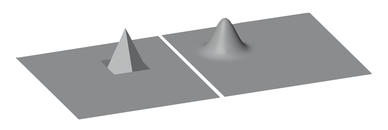
Figure 5: DM command smoothing
To wrap all this DM functionality we have a class at DM.py that implements stuff like the pushing and pulling of the actuators, loading of the commands, etc. Also, it assembles a DM from a config json file that specify how many actuators and the circular mask that have to be applied.
Wavefront Sensor
This is the trickiest component of the system and it is the heart of the simulator. It is also the most interesting one to implement because, as the DM, it works by optically simulating the device. The wavefront sensor simulated here is a Shack–Hartmann wavefront sensor and I already talked about it here. It works by sampling the light spatially using a set of tiny lenses and a big CCD that captures each spatial sample. The details are in the link I just mentioned.
In blender, the WFS component is exactly what a Shack–Hartmann physically is. A set of small lenses forming a circular area where the light is “sampled”. Each lens focus
its light rays at a small “detector”. In our case, the detectors are tiny planes (squeezed cubes) that lies bellow each micro lens on its focus position. In a physical real device, theses detectors are simply a square region on a larger CCD (or any other imaging sensor). There lies the tricky part. Up to focusing the light at the sampled spots, blender was doing all the work raytracing the lithe rays all the way to each tiny detector. Now we have to figure out how to “capture” those light rays that hits the detector. In particular, we need to know where the light rays hit each detector (the x,y coordinate of the hit).
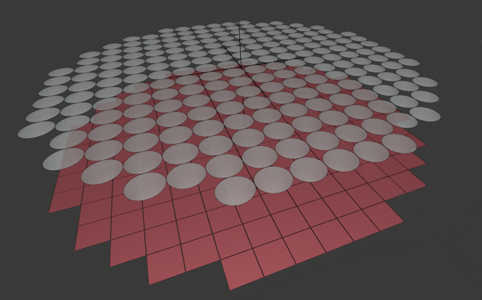
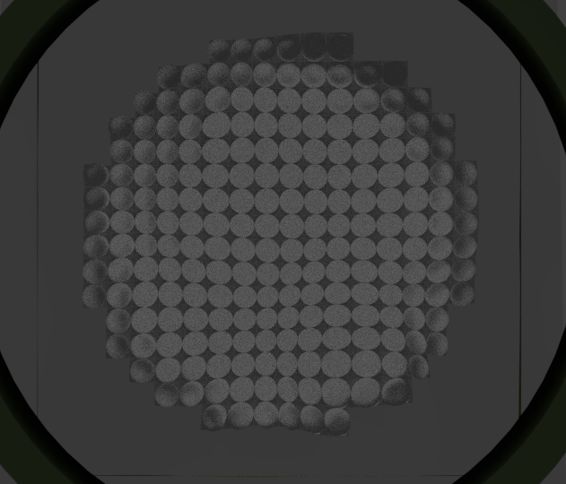
Figure 6: Wavefront sensor component in blender
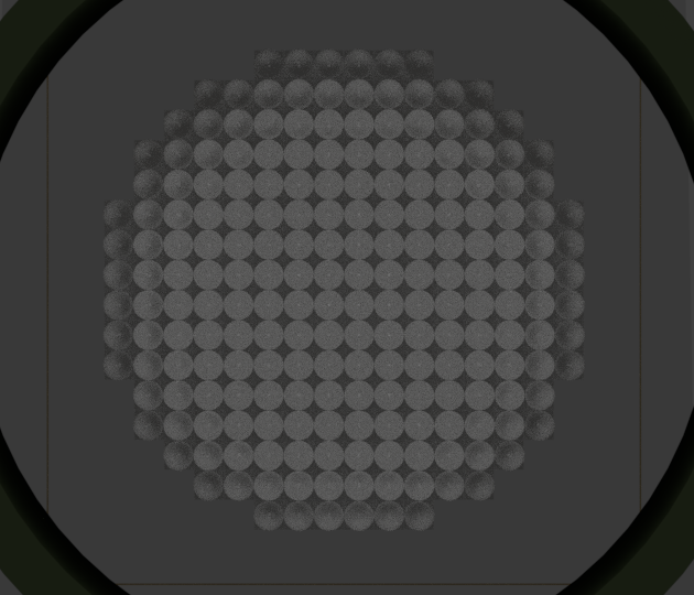
To have an idea what the light path should be, the next figure shows what we would see if we were positioned at the camera. One important point to be mentioned is about the render configuration used in this blender file. As mentioned before, we use Cycles as renderer. Cycles have several parameters that can be configured to produce the appropriate render of an image. Since we don’t use the image that is produced, we basically care about tree of those parameters. The first one is the size of the “image” that would be rendered. Although we don’t care about the produced image, we care about how many rays will be produced. The size of that image influence exactly in how many rays Cycle will generate, hence influencing the precision of our measurement. That leads us to the second important parameter which is the number of rays per pixel. This parameter is controlled by the “samples” Cycles parameter. The third is actually a “set” of parameters and are called “bounces”. They control now many times a light ray can bounce off of different materials. To be able to focus the light on the detector material and simulate refractions, we need to keep the bounces at least 4 or 5 for most of the material properties (reflection, transparency, etc).
|
|
Figure 7: Render of the blender scene from the camera view. Left: Render with a clean light path and no object placed. Right: Same render, but this time with an object placed in the light path.
Now comes the difficult part. The python blender API do not allow us to interact at low level with the render because the rendering have to be SUPER-HYPER fast (and even be allowed to run on the GPU). So, how would we know where the light ray hit the surface of the detectors? Fortunately, blender have a special material where we can code our own “shader” in a special set of C commands called OSL or Open Shading Language. OSL allows us to code, using a C like command language, the way the material threat the light that arrives. For example, if we want an object to appear completely black, we code an OSL function for the material that returns black regardless of where the light hit, intensity of the light, angle, etc. OSL is super cool because you can code crazy behaviour for the material. For instance we can make the material be transparent depending on the angle that the light hits or reflect different colours depending on the place and direction of the light ray (simulating anisotropy). Anyways, we don’t want to create a crazy material. However, using an OSL function as the material for our detector, we have access to the light hit including its position on the object, angle, etc. Up to this point we think that the problem is solved! But unfortunately there is a HUGE drawback. How to communicate this light hit position to the system? Remember that OSL have to be super fast. Because of that, they are compiled BEFORE the rendering starts and they run natively. So, no way to have sophisticated stuff like sockets, memory access, IPC, etc… Everything that happens in the OLS, stays in the OLS…
The solution for this problem was another “gambiarra” which means a set of trickeries involving a lot of different things that usually are NOT meant to be used for that purpose. The first thing was to realise that somehow it should be possible to debug an OSL code. It turns out that you can enable a special debug mode by setting the environment variable OSL_OPTIONS="optimize=0". This will allow us to use a special "printf" inside the OSL to print stuff to the console. Victory!!! There is our loophole! Now, our OSL function is absolutely trivial. It just prints out the position of the light ray out to the console.
#include <stdosl.h>


shader detectorShader(
        output color ColOut = color(0.8))
{
    printf("NIRPS %.6f, %.6f, %.6f\n",P[0],P[1],P[2]);
}
Now, every time we render the screen, the console is flooded with xyz coordinates of light hits. All we have to do is to capture them in the middle of all other console messages. To do that, we start blender using a console pipe to redirect the output as input to another external program that will receive all the prints from blender console and process them. This external program is the python script that we call pipingServer. Now that we have this “interpreter” that receives all blender console, we can send commands to it just by printing it either using python inside blender or using the OSL material we just talked about. Moreover, we have to filter out the normal blender console messages. This is simple enough just by adding some keyword before the prints to identify that we have a string to be interpreted as a command. In our case we prefix all the commands and data with “NIRPS” (which was the name of the project I was working on).
Hence, we need to start blender with the pipe and the filter for the prefix we defined. For convenience, we use a shell script that provide all the typing
#!/bin/bash

PYTHONUNBUFFERED=on

OSL_OPTIONS="optimize=0"

blender main.blend | grep --line-buffered "NIRPS" | ./pipingServer.py
Notice that there are one more configuration we have to make. Either python and grep will try to “buffer” the output / input for efficiency. In our case, this is terrible because we want the command to be processes immediately. This is simple to solve by adding --line-buffered to grep and setting python’s environment variable PYTHONUNBUFFERED=on.
By doing all that, it is possible not only to gather data form the wavefront sensor, but to have a way to send commands to the external python script where we can plot and compute stuff.
Python module and external plots
As mentioned before, we have this pipingServer that receives commands and data from blender. This a straightforward infinite loop that reads an input and processes it. The main loop looks like the following
while "forever":
    # get a line message form blender output
    text = input()

    if text[0:5]=='NIRPS':
        # if message starts with NIRPS, its ours
        text = text[6:]

        if text[0:4] == 'SAVE':
            # just save data without processing
            doSave(x, y, cx, cy, calCx, calCy, filename)

        elif text[0:4] == 'FILE':
            # set filename to save
            filename = text[5:]


        elif text[0:5] == 'PRINT':
            doPrint(x, y, LIMx, LIMy, cx, cy, calCx, calCy)

        elif text[0:4] == 'PROC':
            # Save data to Matlab
            doSaveData()

            # process light hits to find center
            doProcess(x, y, cx, cy, N, data, LIMx, LIMy)

            # save centers
            doSaveCxCy()

        elif text[0:3] == 'CAL':
            # perform calibration
            doCalibrate(calCx, calCy, cx, cy, LIMx, LIMy)

        else:
            # if starts with NIRPS but its just numbers, append to data (they are light hits)
            data.append(list(map(float, text.split(','))))

    else:
        # ignore blender normal console output
        print('[ignored]: '+text)
On this script, no sophisticated math trick is done. It just prepares the RAW data to be used in another script (this one in Matlab) that does the heavy duty math. One of the important commands is the CALIB command. It takes the RAW light hits in the form of xyz coordinates and computes the centroids that will be used as “neutral” sub apertures center. These are the centers that the light rays hit if there is no object in the light path. The interesting thing is that we can calibrate with anything in light path and the system still works (because of the calibration step) as long as the object remains in the same position after the calibration.
Another thing that this script do which is very important is the RAW plots. One of the commands, the PROC command, calls a function that performs a set of very informative plots.

Figure 8: Example of the python plot window
- Light hits: The first one is a scatter plot of the RAW light hits. It shows where the light rays arrived in the 2D surface of the detectors.
- Wavefront slopes: The second one is slopes measured from the current calibrated centers to the last light hits. These indicate the phase distortion that the light suffered when passing through the material in the light path.
- Wavefront magnitude: This one is just the magnitude of each slope in the second plot. It serves only to visually indicate how bad is the distortion suffered by the light. However, this plot might be misleading since we ca have all slopes with constant magnitude but totally crazy slopes angles.
- Phase image: This one is a but trick to explain… This is actually the phase of the light that arrives at the detector. Not to be confused with phase slope. The phase is literally the displace in time the light (measured in phase angle) that the local light wave is taking to arrive at the detector. One might think: How the HELL do you measure the “time” that the light wave takes to arrive at the detector???? If you are wondering that, you:
1 – Have a good grasp of the physics involved. You have this good grasp because you need to understand well about physics to realise that this is something almost impossible to measure easily. Moreover, what do I mean by “wave”??? Wasn’t we simulating the light “RAYS”? To simulate light at the wave level requires us to go much much deeper in the rabbit hole! (if you want to go deeper in the rabbit hole, I have a post about simulating light at the wave level 😅.
2 – You didn’t read the first part of this post and/or didn’t read the post about wavefront sensing 😅. - Point Spread Function: This is the PSF of the last measurement (system + object in the light path). In another words (if you didn’t read the last post %-) its the point of light that we would see if we were in the focus of the system in the position of the WFS. This is not made by discrete light rays, but its the reproduction of the waves of light (yes waves) that hit the detector!
- Image: Finally, this is the image that you would see if we were looking at a NIRPS logo far far away. You see it blurry and distorted because, in this example, there is a random atmosphere in the light path.
Matlab module
This part of the system is implemented in Matlab and does the more specific AO math business like compute interaction matrix, decompositions, Zernike, etc. It starts by reading the the files (data) written by the pipingServer. After that, the first thing we have to do is to compute the interaction matrix. The data need to do that is more than just a calibration data as mentioned before. As explained in the previous post, we need to pinch the DM in several positions to gather enough data to build the interaction matrix, command matrix, command/slope matrix etc. In the blender interface, there is a command that makes blender do all those measurements. This button is called “Command Matrix”. When we click this button, blender produces a pinch of a certain amplitude in each actuator at a time and measure the slope corresponding to each actuator pinch. For each actuator it saves a file in the /tmp folder called DM_i_j.m where i,j is the index of the actuator. Those are the files that Matlab uses to gather data to assemble the interaction matrix. One important thing to notice is that this is the same procedure that a real system does to calibrate the DM/WFS. Again, this is awesome because it means that our simulator does not use any math trick to “emulate” the behaviour or a AO system. Instead, it really simulates the real process! The following figure shows a small animation of the DM pinch calibration.
Figure 9: Calibration of the DM.
After calibrating the interaction matrix, the next step is to read the last measurement (normally with an object in the light path). This will be the measurement that will be corrected by the DM deformation. Hence, the next step is exactly to compute the DM commands that corrects for the last measurement. After computing the mirror commands, they are saved in a text file and is ready to be read back in blender.
With the commands computed and saved, we can go back to blender and load the mirror commands. The commands will be applied to the mirror by displacing the actuators in the same direction that they were pinched during the calibration (perpendicular to the mirror surface). Since the displacement are really small, in order to visualise the commands, a colormap is applied to the mirror to indicate how much each area of the mirror is deformed. After loading the commands, we can perform a new measurement. Now the measurement will take into account the deformation of the mirror and the deformation due to the object together. If everything goes well, one should cancel the other and we should see a sharp PSF in the plot window as well a 0 slopes like it was just after calibration. In other words, the mirror should compensate for the deformation of the light due to the object in the light path.
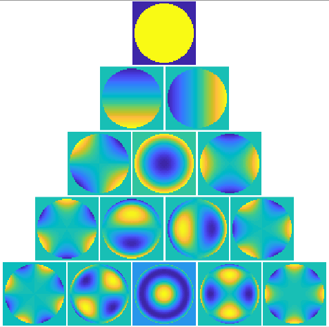
Moreover, the Matlab script also computes a lot of side information used during the process of computing the mirror commands. All of that data are ploted in several windows. We can see the original slopes vs the mirror correction, interaction matrix, command matrix, etc. Another piece of information that is ploted are the modes of the interaction matrix. It is possible to see the zonal as well as the KL modes and its corresponding slopes. The next figure illustrate some of those plots:
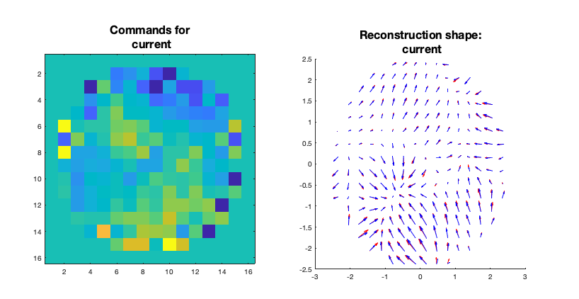
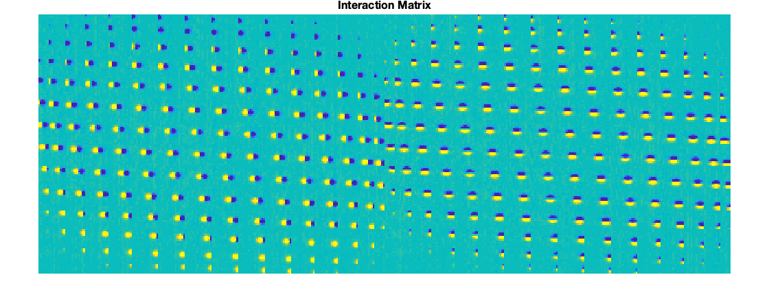
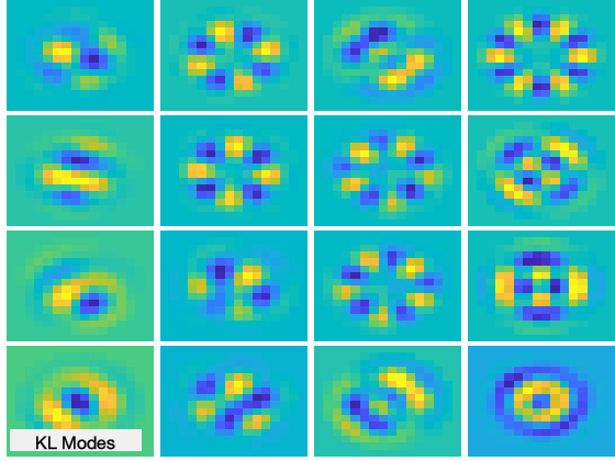
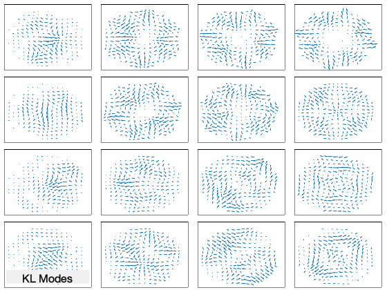
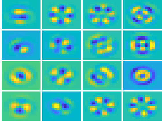
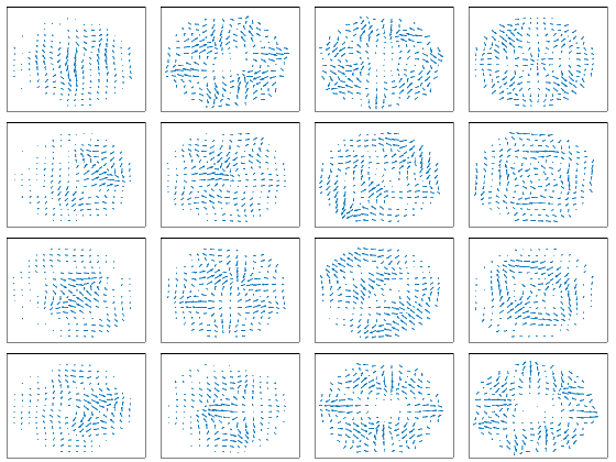
Figure 10: Plots resulting of the Matlab computation of the DM commands. DM commands, Interaction matrix, KL modes and slopes, Zonal modes and slopes.
Results
To illustrate some results, here we have two examples of the performance of the system. In each one, we put a different object in the light path. Then, we proceed with the computation of the DM commands that corrects for the deformation produced by that object. In the end we compare the PSF before and after the correction. In both samples a sequence of pictures are presented that are, up to this point, self explanatory.
The flat calibration
As mentioned in the previous sections, before doing any measurement, we need to calibrate the system. The calibration is done with the light path empty as shown in the following figure:
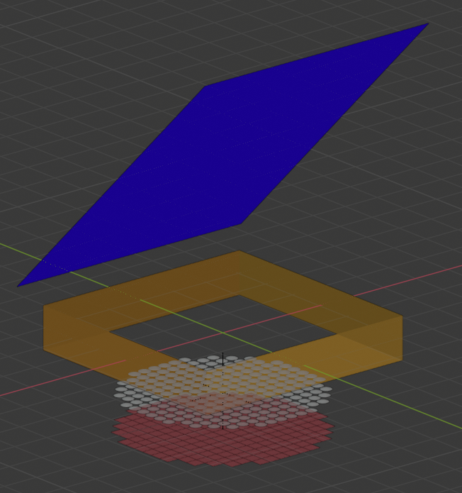
Figure 11: Light path during calibration. The orange square is the region where we place objects. For the calibration it must be empty.
As a result, we have perfectly flat slopes and the PSF is perfectly sharp (except for the diffraction limit as explained in the previous post).
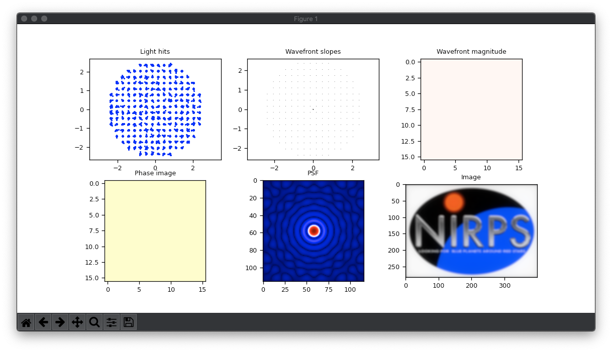
Figure 12: Plots result for the calibration. Everything looks flat and the PSF is diffraction limited.
Simple geometry example
The first result is a toy example that uses a very regular shaped object. The goal is to see how the system corrects for extreme distortions.
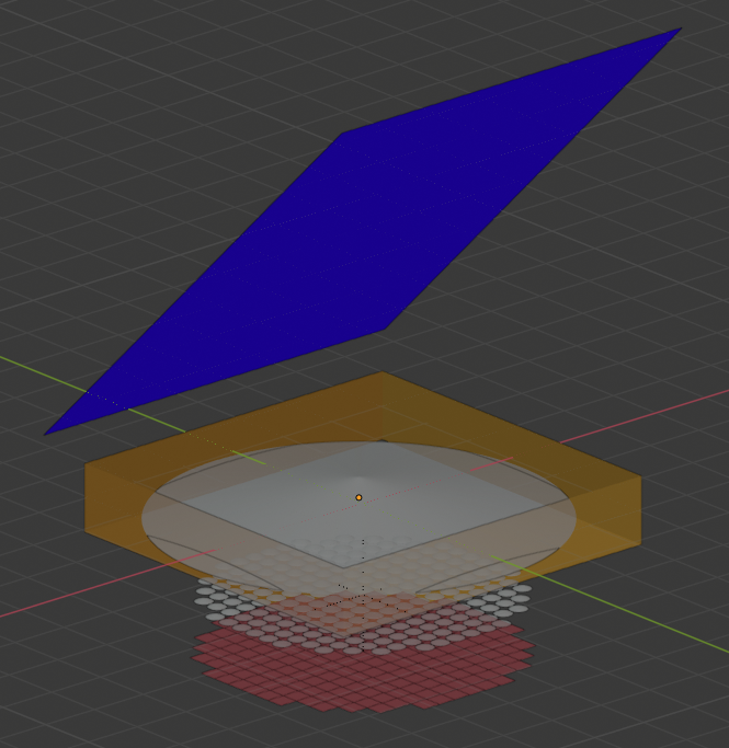
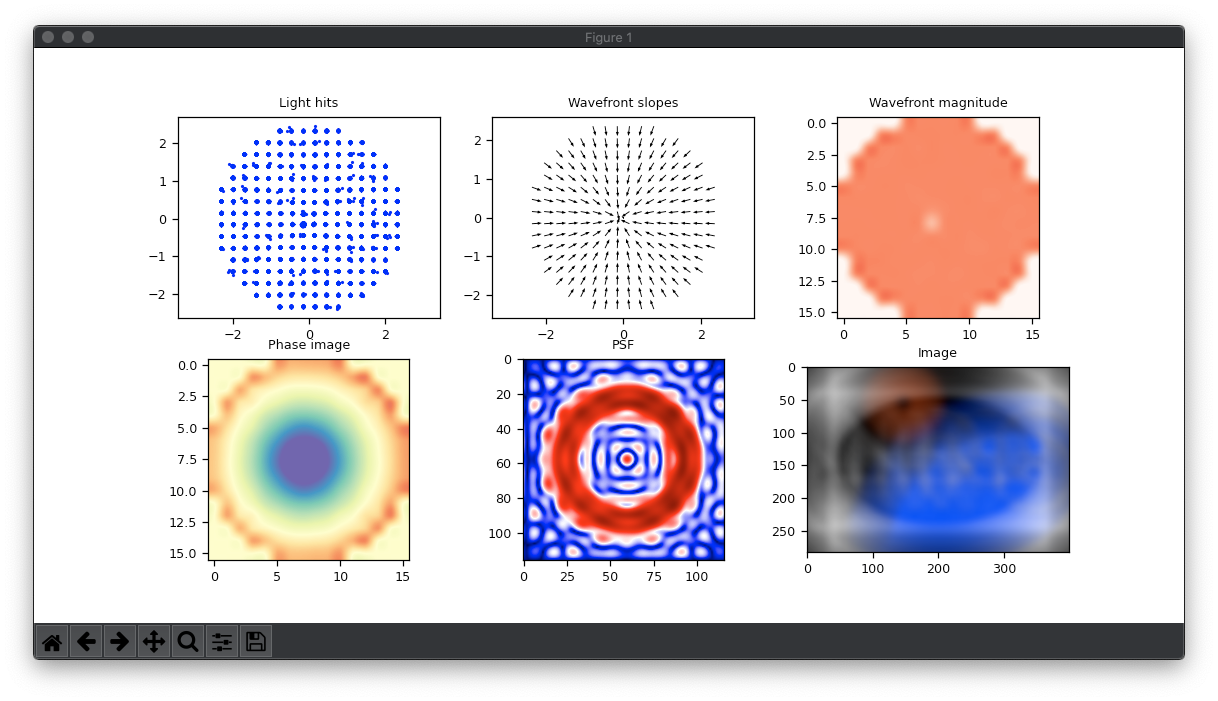
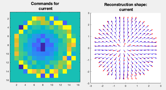
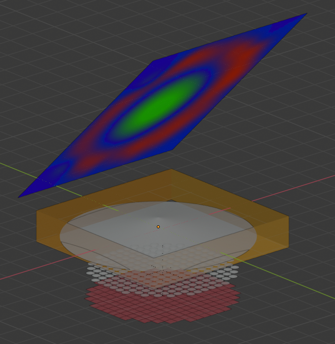
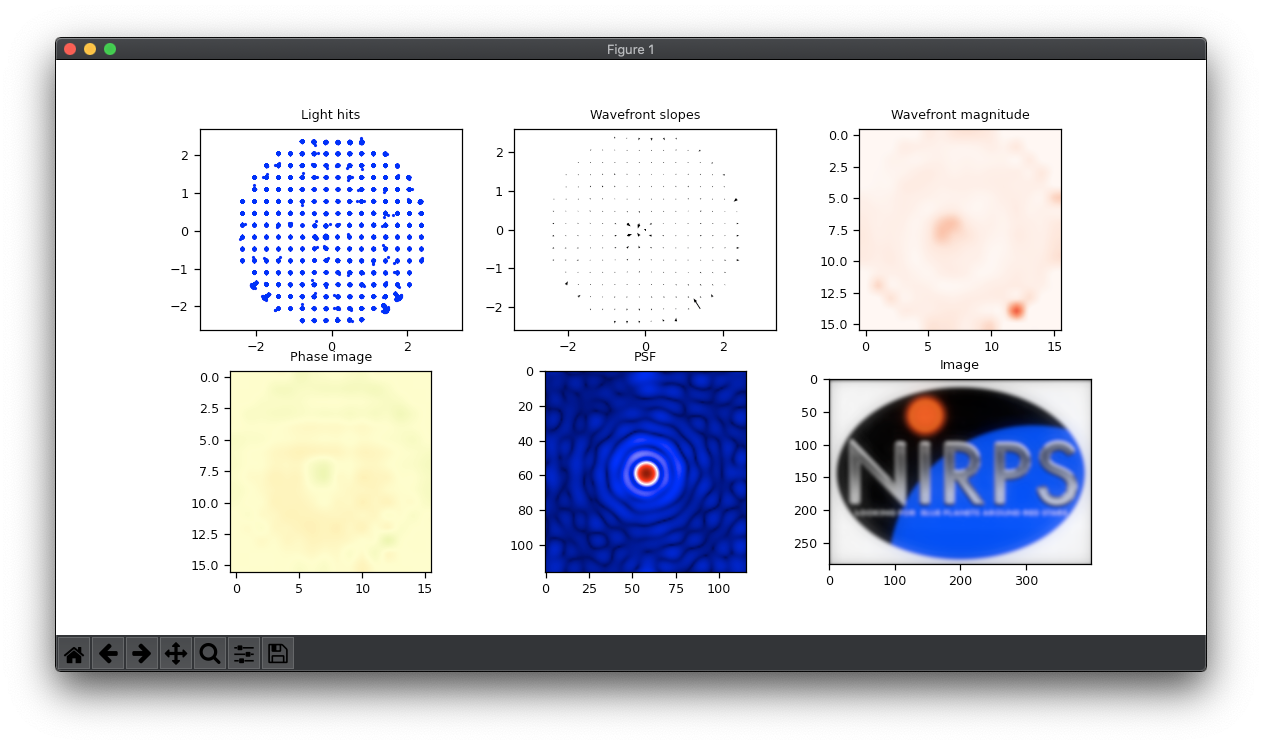
Figure 13: Results for a basic transparent cone. From top to bottom: 1 – Object in the light path with flat DM. 2 – Measurement plots for the object. 3 – Computed commands for the DM. 4 – Object in the light path and DM with loaded commands. 5 – New measurement showing the correction.
Atmosphere simulation
In this second example we try to simulate a fake atmosphere by using a “irregular and noisy” object. We make this object “elongated” on purpose (see next section bellow) so we have different atmospheres just by moving the object in front of the light path.
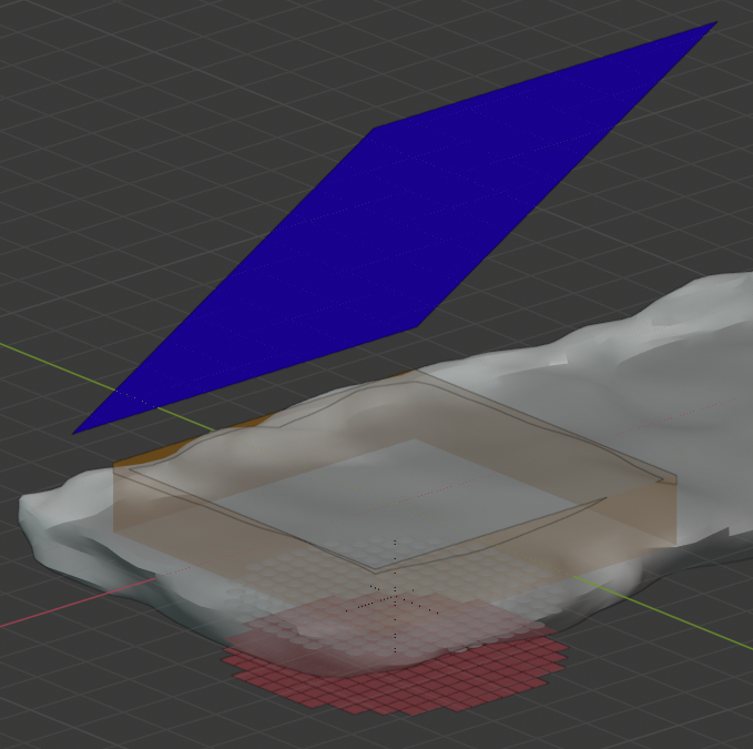
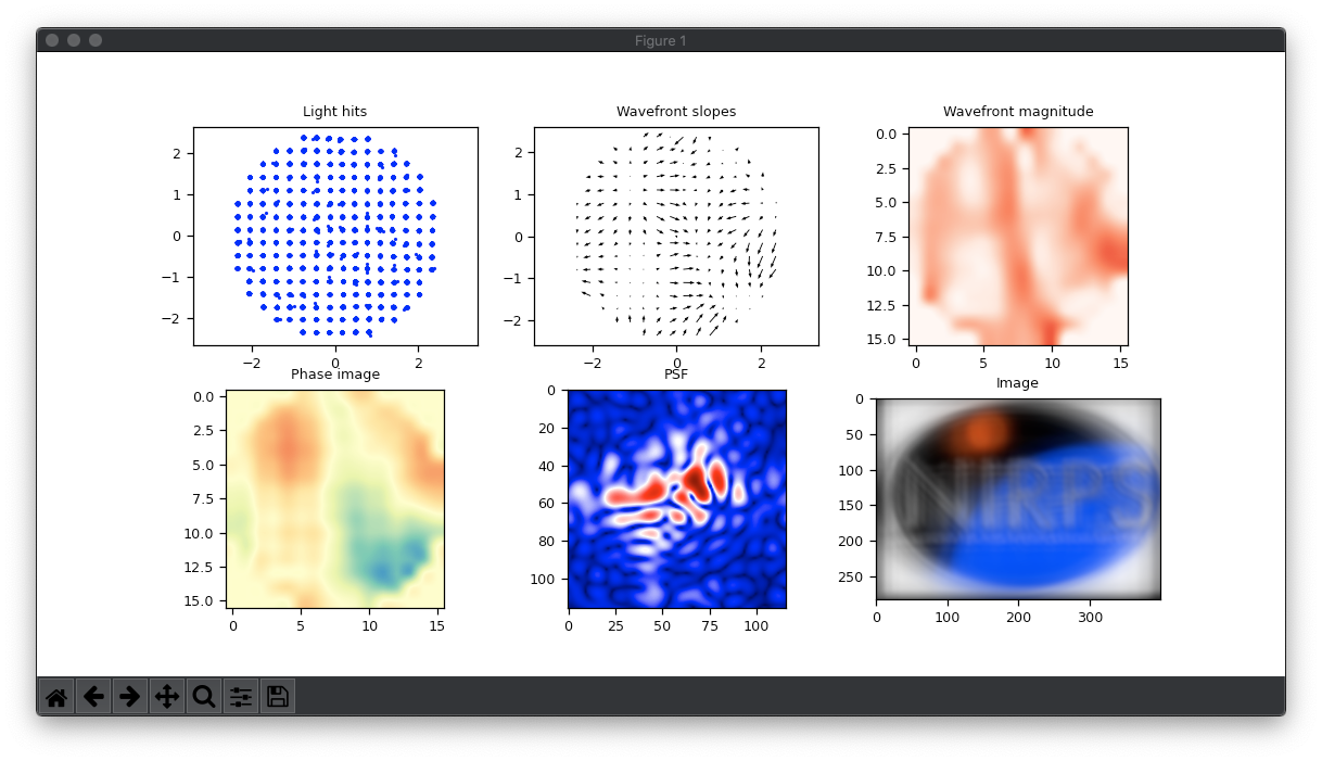
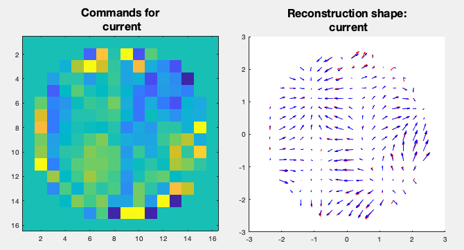
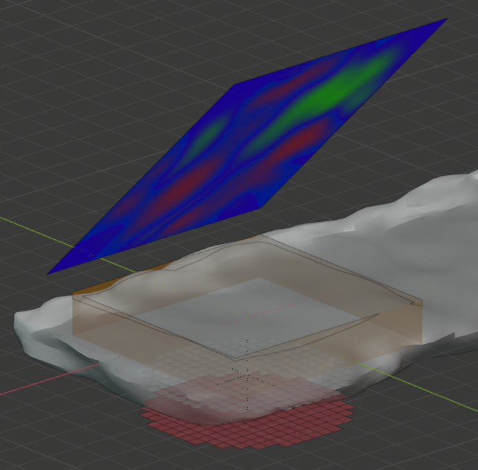

Figure 14: Results for a simulated atmosphere. From top to bottom: 1 – Object in the light path with flat DM. 2 – Measurement plots for the object. 3 – Computed commands for the DM. 4 – Object in the light path and DM with loaded commands. 5 – New measurement showing the correction.
Extra bit
Just for fun, we implemented a special loop in blender that moves the atmosphere object by a small amount each time. Each time, it performs a measurement and saves the resulting plot. By doing that for several iterations, we end up with a small animation of a simulated atmosphere in action. So, by looking at the PSF we see the same effect we have when we look at a star in the sky. You can see this animation in the next video.
Figure 15: Atmosphere simulation using the system
Conclusions
This was a really fun project. I had to learn a lot of stuff and apply math concepts in a very practical way. As I mentioned in the previous post, I didn’t really use this simulator for anything serious, but it was very useful for me to understand the concepts I was immerse on. As always, that you for reading up to here. The code and files are on GitHub and if you have any question, critic or comment, please leave it on the comment section bellow. I would love to talk about it!