Introduction

In this post I’ll talk about one of the most amazing algorithms I ever came across. HashLife. I’m a bit suspicious to call this one the most amazing one because it deals with another thing that I find absolutely amazing. Game of Life (GoL for short). In short, HashLife is an algorithm that speeds up the computation of the GoL by factors of thousands, millions, billions and, as a matter of fact, as much as you need it to (and have resources to do it). As always, the source code is available on GitHub.

I’m making this post a bit “late” because since I met this algorithm, years ago, I always wanted to implement it but never had time to understand it fully. I came across it in a software called Golly which is a program to edit/construct/simulate Game of Life patterns. Before Golly, I already had my own implementation of GoL, but using the naive implementation that is really slow. Because of that, I did not knew about its true potential. That’s because large patterns took forever to evolve and show some really shocking behaviour. But with Golly, I could open huge pre design patterns. Really big ones. When we clicked play, as expected, they took forever to evolve. However, there was a small button with a lightning bolt on it. When we click it, something magical happens! After a few seconds, the patterns jumped tens, hundreds, thousands some times millions of generations ahead in a matter of milliseconds!!!! You would guess the small label hint that appear when we hover the mouse of it: Hashlife. After that discover, I kept googling for this magical word and found out that its the name of a awesome algorithm that make GoL even more magical for me!

Throughout those years, form time to time, I use to spend a couple of hours trying to understand that algorithm but gave up because I thought was too complex. During those moments, I stumble across a couple of articles talking about the algorithm (beside the original paper). One in particular, was very very useful for me to understand the algorithm: “An Algorithm to Compress Space and Time” by Tomas G. Rokicki. He sounds like a very very smart guy and I love his post. Later on I found out that he was one of the authors of Golly (no surprise %-).

His article is far far better than this one, for sure! And I wouldn’t dare to even try to do better. However I’ll try to give a bit more details about how the algorithm works, probably just because I’ll put more pictures and talk more about it 😅. Nevertheless, if you really want to understand this amazing algorithm, you should read his article. Another important aspect is that, in his article, he said everything I wanted to say about the algorithm. Things like the way it speeds up time using hashing mechanism, how quad trees do the space compression, etc. Even his title is the best one could think! So, thank you Dr. Rokicki for the great article.

As I mentioned, I’ll try to give a bit more details in this article. Moreover, I’ll try to follow what I consider being the intuitive thinking when one try to implement the Hashlife algorithm. This will lead to dead ends that are normal when we try to implement something that is non-intuitive. The hope is that, by showing my thinking process, it will be useful and didactic enough for you to understand and implement your own version.

Game of Life

There is no point in explaining what HashLife is without explaining what GoL is. After all, HashLife is an algorithm to speed up GoL.

Game of Life is not a game 😅 (at least in the common sense of the word). It is a construction invented by John Conway that involves an infinite square grid of cells and a couple of rules. Technically, GoL is an automaton.
In this “Game”, each square of the grid is a cell that could be in two states, “dead” or “alive”. The rules dictates what happens with the cells as time goes by in steps. At each time step, the only thing that can happen is the cell to stay as it is or change its state. Hence, a dead cell can remain dead or come to life, as well as a live cell can stay alive or die. Those behaviours are dictated by the rules. Thats it. GoL is basically this grid evolving in time. In each step, all the cells of the grid are tested against the rules and could change state or not. In the traditional GoL, the rules a very simples:

• Any live cell with two or three live neighbours survives.
• Any dead cell with three live neighbours becomes a live cell.
• All other live cells die in the next generation. Similarly, all other dead cells stay dead.

Yes, these are the only 3 rules. So, you start with the whole infinite grid as dead cells. You manually change the state of some cells making some pattern of live cells. You start the GoL on this grid and see how the cells “evolve”. There are plenty of online GoL simulators where you can “draw” your own pattern and see the animation of how it will evolve. In fact, you can easily implement your own GoL animation by fixing the size of the grid (say 1000 x 1000) and implement a loop in which, at each step, goes through all the cells in the grid testing the rules for each one, applying the change when necessary. Or, if you want, you can try yourself in the next figure/applet…

Figure x: Game of Life

If you never heard of GoL before, you must be wondering: what the heck does one find interesting about this thing at all?!?!. Without HashLife, the answer to this question would not be so compelling. To start, whiteout HashLife, you can at least see why they called “life”. If you draw some random pattern in the grid and evolve it for some steps (by the way, steps are called generations) you will notice that the cells behave in a kind of “life like” behaviour. This alone was enough to amaze me in the past. With such simples rules, you already see patterns that oscillate, “glide” or walk and evolve. Moreover, if you tailor carefully enough the initial pattern, you can see complex patterns like “guns” (patterns that generates other patterns), “puffers” (patterns that shoots random cells), etc. All that, from those 3 innocent looking rules. As I said, up to this point, you don’t need HashLife. With a naive “grid scanning” implementation you can see those behaviours in hundreds or thousands of generations.

There is a whole community around GoL. People even use it for serious research in pure math. It is such, that there is even a “Life Lexicon” dictionary to name standard patterns. Actually, as I said before, the technical designation for GoL is that it is an “Automata”. People study this stuff a lot in Computer Science and Mathematics. For instance, we can change the rules and study properties that might arise from those new rules.

HashLife

As I said before, HashLife is an algorithm that speeds up the computation of the GoL. In particular, it allows us to skip generations ahead and evolve the grid thousands or millions of generations in one step. Moreover, and at the same time, it does that in a very efficient memory representation of the grid. So, in essence, it is an algorithm to compress space and time (as the great article from Dr. Rokicki states already in the title 😄). The algorithm itself was not invented by Dr. Rokicki, it was created by a guy called William Gosper and published in a paper called “Exploiting Regularities in Large Cellular Spaces” on Physica 10D, 1984. Unfortunately, Bill Gosper (as he was most known), did not write the paper for a brother audience. It is a Physics paper, so there is little information about the algorithm itself, just the idea. But, fortunately that was enough for people to implement it and make it somewhat “famous” (although you might count in the fingers of one hand, articles like this, explaining in details the algorithm).

So, how does one speeds up a computation by a factor of one million??? Moreover, how can this be done not only in time but in space also??? This is where the paper from Bill Gospel is most useful because he gives alway in the title fo this paper: “Exploiting Regularities in Large Cellular Spaces”. The key point here is “Regularities”.

We will look at the two aspects of the algorithm: Space and Time. The two magical words here are “Quadtrees” (for space) and “Hashing” (for time). To better explain how the algorithm speeds up so much (and takes so little memory space), I think is useful to show, first, that this is indeed possible in the GoL. In the next sections we will take those aspects, space and time, separately.

Space compression

This is the easiest of both aspects. To show that is possible to achieve tremendous compression, we can take a trivial example. We could represent an empty 1000×1000 grid by just the size and the content “0” (1000, 1000, 0), so, with 3 numbers we would be representing a one million points grid.

But of course this is a silly example because is too extreme. As I said before, the magic word here is quadtree. The idea of how a quadtree works is that you start from a finite power of two sided grid (say 256×256) at “top level” and go one level down by dividing it into four (“quad” from Latin I guess) 128×128 “sub-grids”, then, each of those you divide again into 4 and so one and so forth until you reach a minimus size block. We now have the first characteristics of the HashLife algorithm: It works on grid. In another words, the grid will have to have a power of 2 length. The following figure illustrates the process.

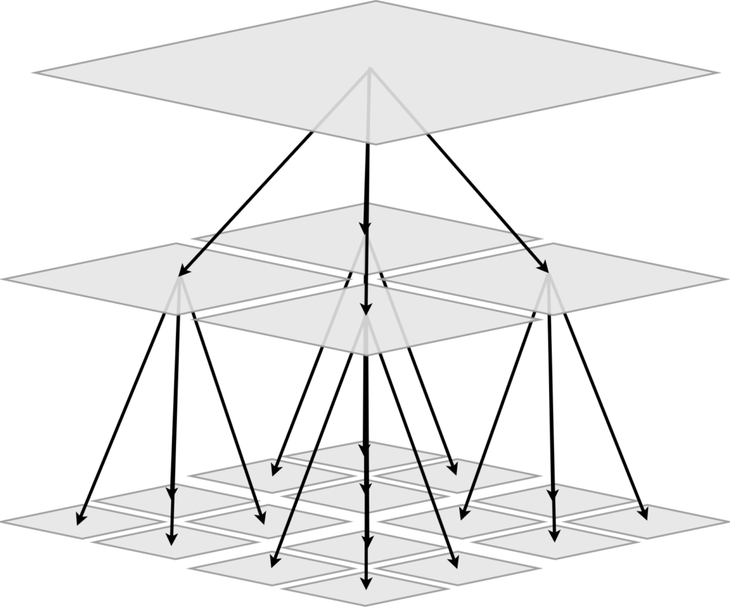
Figure x: Concept of a quadtree division mechanism

In the original “quadtree compression”, you stop dividing every time you see a completely uniform block and keep dividing otherwise. The next figure show how this compression would work to store a pattern, As you can see, the original big block is stored as a set of small ones.

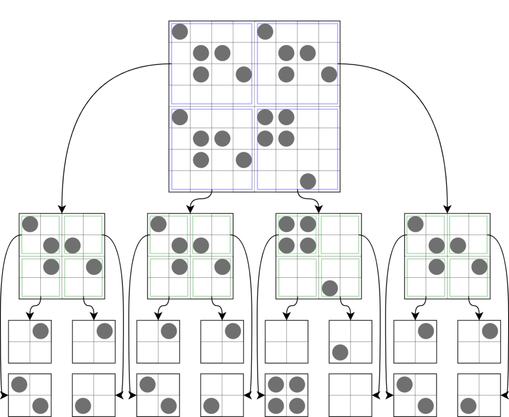
Figure x: Example of a quadtree division for a pattern

In hashLife we have more or less the same idea. We keep dividing until we reach what we call “canonical blocks”. Those canonical blocks form a set of blocks that can be used to form anything (like a basis in linear algebra, for those who are more into math).
For instance, we can “canonize” all the possible 2×2 cell blocks. With that, we are going to have 16 possible 2×2 blocks from a completely empty/dead 2×2 block to a completely alive/full one. With those 16 blocks we can build any pattern. Hence, to decompose a given complex pattern, we perform the quadtree division until we reach lots of 2×2 blocks.
Now, each block larger than a canonical one is made up of pointers to blocks one level down until reach a canonical block. The next figure shows the process. You can see the quadtree division and then the pointers to the blocks. Notice now we don’t store the block itself anymore. Instead, we store pointers to smaller blocks. Moreover, we can “cache” similar blocks to optimise the space. From now on we will call block as “nodes” because now they are represented as the same data structure regardless of the level they are on.
As an example, a 1024×1024 block would be represented by a node that have 4 pointes to 4 other nodes that, each will have 4 pointers, etc, etc, etc. If that big block had many repeated patterns (like empty areas for instance), you need only to store one of the empty areas and all the others would be just pointers to it.

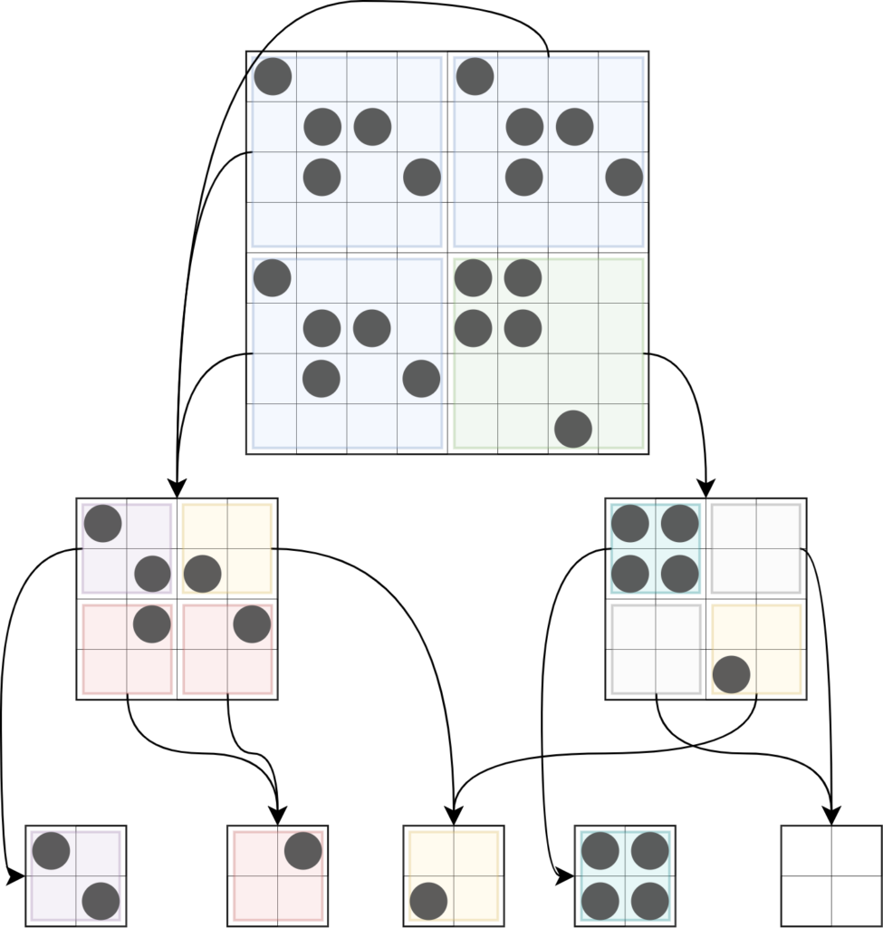
Figure x: Quadtree compression

With that, we reach another very important aspect of the HashLife algorithm: the definition of a node. As I explained before, a node will represent a block at some level. Hence it will be a data structure with some properties. Following, we have the definition.

class Node:

    def __init__(self, sw, se, nw, ne):
        self.sw = sw
        self.se = se
        self.nw = nw
        self.ne = ne
        self.depth = 0
        self.area = 0

The node can have more properties to deal with some technical details (that I’ll explain later). For now (and for simplicity) we just need to understand that code snippet. First we have four properties called sw, se, nw, ne. These corresponds to pointers to nodes in the four quadrants, namely the south-west node, south-east node, north-west node and north-east node. depth is the level or how deep this node is in the full representation of the quadtree. Finally, area is not needed for the algorithm itself but it will help a lot for some adjacent processing that I’ll explain later.

Hence, in HashLife, a GoL grid is now represented by a single node with some depth and pointers to other nodes one level down. Moreover, if a node is at level 1, it is a canonical node. In this case, and only in this case, the properties sw, se, nw, ne are not pointers, but numbers: 0 meaning a dead cell and 1 meaning a live cell. Also, if the pattern has high degree of regularity, meaning that it has repeated sub patterns in it, the size of the data structure will be small because each repeated block will be represented by the same pointer.

At this point, it is very very important to have a convention on your head for the sequence in witch you will describe a node with its sub-nodes. In my case, I started from the bottom left (sw node) and went left to right to then go up (and back to left). Hence, my sequence is showed in the next figure. Its important to understand that this sequence has absolutely no impact on the implementation, it serves only to facilitate YOUR thinking. As you will see, there will be parts in the code where you will have to break down and reassemble nodes very often. This sequence helps to mentally do this job and code the right node breakdown.

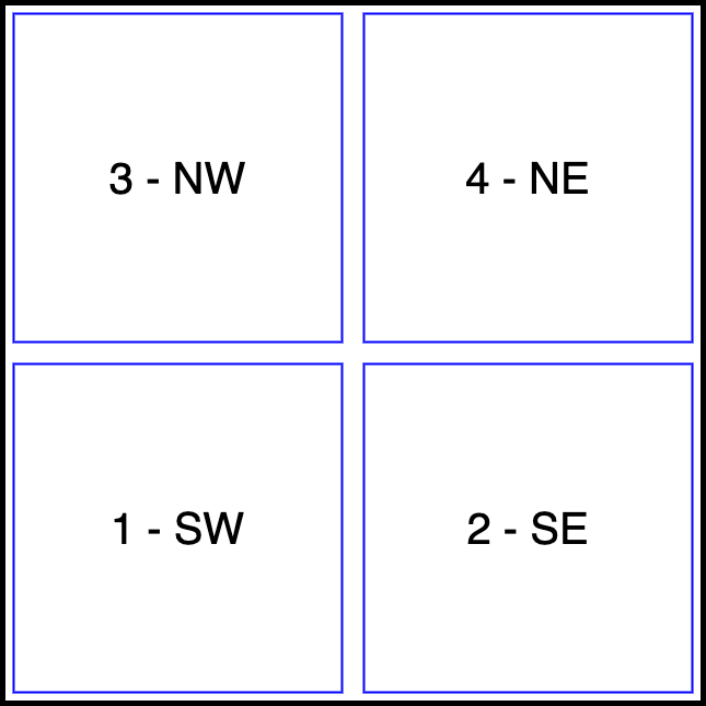
Figure x: Node names and sequence convention.

Evolving the rules in compressed space

All the quadtree business is really nice and allows us to have really large patterns stored in a very efficient way. But there is one big point that needs to be explained. What is the point in compress it if, to apply the rules, we need to test each individual cell? If we have to decompress every time to apply the rules, what do we gain? The answer is: We don’t! We apply the rules on the compresses data structure!!!

Up to this point, we don’t have anything about how the the Hashlife algorithm evolves the grid. The first impressive thing that it does is what I mentioned before: To evolve the compressed pattern without having to inflate or decompress the quadtree! The basic idea is, in principle, simple. The quadtree notion leads us to think recursively. You have a big block, you call a function to divide it, and call itself on the four pieces, recursively. This is more or less the idea. Lets call the function that performs a GoL step on a block “evolve“. It receives a square grid and apply the GoL rules on the cells. Now we could think on making a recursive version of this function. In other words, the function would call itself on the 4 divided blocks until a minimus size is reached. It would looks like something like the following pseudo-code:

def evolve(node):
    
    if node.depth==2:
        return evolve node using GoL rules
    else:
        res1 = evolve(node.sw)
        res2 = evolve(node.se)
        res3 = evolve(node.nw)
        res4 = evolve(node.ne)
        
        res = assembleCenterNode(re1, res2, res3, res4)
        
        return res

Unfortunately this pseudo-code has a huge drawback. To evolve a node, you need its neighbours (at least one extra row and column each side). Although one could think of ways to go around that problem, most of the solutions would not provide the structure needed for the second part of the algorithm, which is the “time compression”. The way that was idealised by Bill Gosper was the following;
We create the concept of “center node”. Basically, each node now has a central region where we will compute the result. Now the algorithm takes a node and returns a smaller node one generation ahead. The next figure shows the geometry of this scheme.

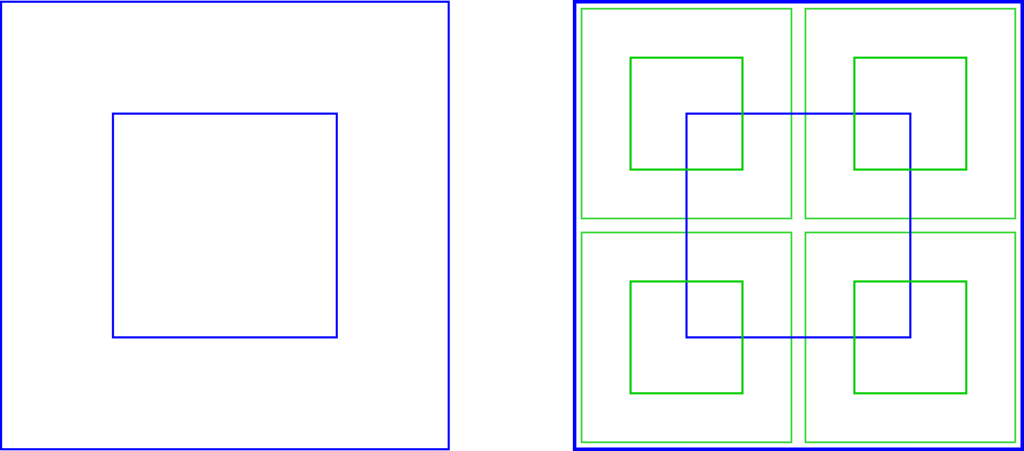
Figure x: Center node representation. Each node has a center region where we ensure that the result (next generation) will be computed. We still perform the quadtree subdivision, but each level the nodes also have the concept of center node. The center node has half the size of the original node (half of the width and half of the length) and it is perfectly centred.

In summary, the function evolve receives the node at level depth and returns a new node at level depth-1 because it has half of the size of the original node. One important thing is that, although physically this result was centred in the previous node, there is no concept of “position” for the new node because its position if defined by the links to the subnodes and its parent. Its just a new instance of the class node which happens to represent the GoL next generation for the previous larger block. The only meaningful position for a node is wether it is the north east, south west, etc, of a parent node.

Another very important aspect to point out is that the result of each step is a smaller node. Hence, we cannot just keep evolving by calling the function on the previous result. This will quickly shrink the result to nothing. Fortunately this is very simple to solve. At each iteration, we add an empty “border” to the topmost node (called root node) creating a new root node with the original node in middle. Now the loop of the generations is something like this:

• Get a node of depth d
• Add an empty border generating a node of dept d+1
• Get the result of one iteration as node half of the size (depth (d+1)-1 = b
• repeat

Up to this point, we know about the center node and the high level approach of having a function that receives a node and returns a smaller node with the result. The problem now is that this center node is “spatially not aligned” with the quadtree geometry. If you look back to the previous figure, you can deduce that the center node is composed by parts of the sub-nodes (north-east, north-west, etc) of the original big node. When we call the evolve function it have to compute this center region result. As we mentioned before we can’t just call evolve on each subnode because each one would result only their center nodes. In the previous figure, the blue node is the node we are calling evolve on, and the green ones are its subnodes. Notice that if we just call evolve on each green nodes, the results would be just the green centres and we would now have enough information to assemble the blue center node.

To solve this problem, we create 9 auxiliary nodes showed in the next figure as red nodes. Those include the original subnodes and 5 more positioned in such a way that they results could be combined to form the center result of the original node.

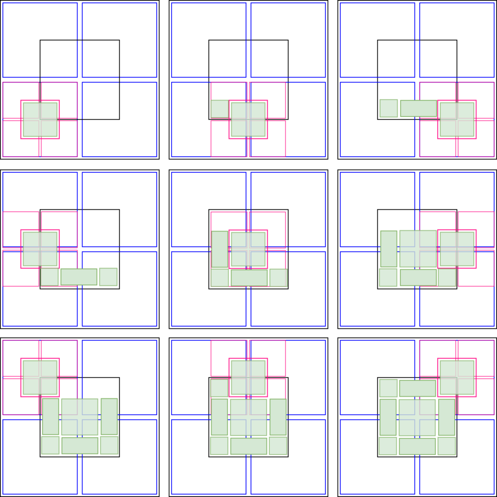
Figure x: Composition of the center node from the results of the 9 auxiliary nodes. The original node we want to evolve is the big black node. Its subnodes are represented by the blue nodes. The auxiliary nodes are represented in red (along with each of its corresponding subnodse). Each red node have its center filled in green to illustrate their result. They are showed in a sequence for didactic purpose. As we compute the result of each auxiliary node, we can use part of this result to assemble the final result which is the center of the black node.

Now we can update our evolve function as the following pseudo-code:

def evolve(node):
    
    if node.depth==2:
        return evolve node using GoL rules
    else:
        node1 = Create Auxiliary Node 1
        node2 = Create Auxiliary Node 2
        node3 = Create Auxiliary Node 3
        node4 = Create Auxiliary Node 4
        node5 = Create Auxiliary Node 5
        node6 = Create Auxiliary Node 6
        node7 = Create Auxiliary Node 7
        node8 = Create Auxiliary Node 8
        node9 = Create Auxiliary Node 9

        node1Res = evolve(node1)
        node2Res = evolve(node2)
        node3Res = evolve(node3)
        node4Res = evolve(node4)
        node5Res = evolve(node5)
        node6Res = evolve(node6)
        node7Res = evolve(node7)
        node8Res = evolve(node8)
        node9Res = evolve(node9)

        result = assembleCenterNode(node1Res, node2Res, node3Res, node4Res, node5Res, node6Res, node7Res, node8Res, node9Res)
        
        return result

Now we have a working algorithm. Unfortunately its not over yet 😅. As it is, this algorithm performs one step of GoL in a compressed grid. This is already awesome. Now it is possible to evolve a really large pattern in a compressed manner and perform a step on it without even decompressing it. This is considered a “space optimisation” of the original GoL algorithm. Before we jump on the “time optimisation”, we need to make a small change in the code.

Although the current pseudo-code works, we will add an extra set of steps that will prove to be key for the time optimisation later. This modification deals with the way we re-assemble the resulting center node using the results of the 9 auxiliary nodes. If you look at the previous picture, we could use the green nodes to compose back the black center but that will involve breaking down the nodes a lot. For instance, if we call the black center resulting node as res, the lower left corner of the resulting green node will not compute the full res.sw. Instead, it will actually compute only res.sw.sw. Moreover, if we call the green resulting node as res1, the little green tile that will form res.sw.sw will be actually res1.ne.sw. An so on…

Instead of going through all the sub-sub-nodes breakdown, we get the 9 results and assemble 4 intermediate nodes showed in the next figure. Notice that this procedure seems unnecessary and is, in fact, a bit redundant since we use the same auxiliary node more than one time to assemble this 4 intermediate nodes. However, as I mentioned before, this will be a key point for speed later on.

Figure x: Clever strategy for assembling the center node quadrants. This assembly will allow the hyper-speed to be computed.

Now we have to update the pseudo-code one more time. This time we need an auxiliary function called getCenterNode that received a node, breaks it down, and reassemble the center, returning it as a node.

def evolve(node):
    
    if node.depth==2:
        return evolve node using GoL rules
    else:
        node1 = Create Auxiliary Node 1
        node2 = Create Auxiliary Node 2
        node3 = Create Auxiliary Node 3
        node4 = Create Auxiliary Node 4
        node5 = Create Auxiliary Node 5
        node6 = Create Auxiliary Node 6
        node7 = Create Auxiliary Node 7
        node8 = Create Auxiliary Node 8
        node9 = Create Auxiliary Node 9

        node1Res = evolve(node1)
        node2Res = evolve(node2)
        node3Res = evolve(node3)
        node4Res = evolve(node4)
        node5Res = evolve(node5)
        node6Res = evolve(node6)
        node7Res = evolve(node7)
        node8Res = evolve(node8)
        node9Res = evolve(node9)

        intermediateNode1 = assembleNode(node1Res, node2Res, node4Res, node5Res)
        intermediateNode1 = assembleNode(node2Res, node3Res, node5Res, node6Res)
        intermediateNode1 = assembleNode(node4Res, node5Res, node7Res, node8Res)
        intermediateNode1 = assembleNode(node5Res, node6Res, node8Res, node9Res)
        
        result = assembleNode( getCenterNode(intermediateNode1), getCenterNode(intermediateNode2), 
                               getCenterNode(intermediateNode3), getCenterNode(intermediateNode4) )
        
        return result

Time…

The algorithm so far is not HashLife yet. It is faster than the naive “grid sweeping” GoL implementation just because it computes steps in the compressed data. Hence, for very large (mostly empty) grid, it has to do less computation. But its still normal “1 step” evolution of GoL.

Now, lets talk about speed. I’ll divide the “time optimisation” in two parts. The first part is the intuitive dynamic programming approach of using a hash function on the structure so far developed. The second part is where the real magic happens!

Hash function and dynamic programming

To understand this time optimisation, you need to understand how dynamic programming works. Basically it deals with the concept of “caching results”. The principle is extremely simple and powerful. In a few words, if you have some computation (maybe a function) that receives a set of parameters and returns a result, you can cache this result so that, next time you receive the same parameters, you don’t wast time computing the result again and just returns the cached one. This is some times called “memoization”. This cache can be implemented easily in most cases with a very common data structure called Hash table. I think now its obvious where the term HashLife came from 😅. This procedure is exactly what the first time optimisation is all about. The function that will be “memoized” will be exactly the evolve function. This memoization is pretty simple but require some technical aspects that we should be aware. The first step is to have a Hash table as our cache. Initially, this cache it will be be empty. The keys on this table will be nodes and the values will also be nodes (but the smaller center results). This is the simplest caching mechanism that is. Basically the Hash table will behave exactly as the evolve function. Hence, the first thing we do in the evolve function is to test wether the node we will process is in the Hash table. If it is, don’t do anything and just return the result stored in the Hash for that key. If its not present, proceed normally with the computations we showed so far. However, before returning the result, make sure you add a new entry on the Hash table with the key being the node you processed and value being the computed result. Now, next time the function received this node, its not going to require any time to process.

As with all Hash tables, this one needs a Hash function. Hash function is the function that receives the hash key and computes an address in the internal Hash list that stores the values. In order to make this procedure possible, our node class have to be what we call “Hashable”. This means that if two nodes represent the same GoL pattern, they should return the same value when called in the Hash function. This is easy to implement but not that trivial to analise. Because of the space compression, our nodes are half way ready to be hashable. In theory, we could use the node address as Hash function result. This is due to the space compression procedure of the quadtree structure (equal nodes have equal pointers). Because of it, if two nodes or subnodes represent the same pattern in the GoL grid, by space compression architecture, they are the same node (have the same pointer). However, there is a slight complication… As we saw before, during the process of computing the result, we have to assemble new nodes that are not aligned with the quadtree nodes (for example, the center nodes). Nevertheless, we can solve this problem by making the Hash function that returns some combination of the pointers of the subnodes of the original node. That will allow two nodes that have different pointers but same subnodes representation, return the same Hash function value and hence be considered the same node. This technical strategy of making a node heashable, will allow two nodes to return the same result regardless of its position in the grid.

It is worth to analyse how much speed we can get out of this memoization done in the evolve function. Lets get an extreme case. Imagine a 1024×1024 node that never grows and is periodic (let say it goes back to the initial pattern after generations). Initially, the cache will be empty, but as the grid evolves, more and more parts of it will be cached to the point that, eventually, we cache all the results even for the root node. When we reach this point, no more computation is needed! The whole GoL elocution will boil down to “jumps” in the cache. Hence, no processing is done anymore. The limit now is the memory jumps between the hash table values.

The next applet shows the evolution of two generations using this “slow” Hashlife algorithm. In the next section you will understand why this is still slow 😅. The grid contains a simple pattern (a very famous oscillator). The grid also has lines with different thickness to give us an idea of the quadtree division (but its only for visual aid). You can press the play button or you can navigate back and forth with the slider. During the evolution of the algorithm it will take several (many) steps to complete a single generation. During the evolution, you will see a blue “node” jumping around. That represents the current quadtree node being processed. Notice that it also jumps in places that are “not align” with the quadtree. That happens when its testing the 9 auxiliary nodes in each level. Every time it hits an “unseeing” node (a node that has never being processed), it computes the result and stores in the hash table (caches it). The hash table is presented by the pile of nodes in the right side of the applet. So, each time the blue block visits an unseeing node, it will be cached and a small copy of it will appear in the right side table. In that table, the nodes appear with green and red cells which represent the original node and its result. Notice that we also cache empty nodes. On the other hand, whenever the blue node visits an already visited node, its corresponding hash element blinks blue, indicating that we don’t need to process it, just take the result from the hash table.

Another very interesting thing to notice is that, once the hash table is complete, its nodes keep blinking and the jumps between values takes place. For visualisation sake, I erased the hash table after each generation otherwise I would run out of screen. Needless to say that this is NOT the case in real operation. The hash table only grows and reaches a point where it grows very very slow or even (for periodic patters) stop growing at all.

We can compare the processing cost of this example using this slow Hashlife with the naive approach. This grid has depth of 5, which means that it has 32×32 (1024) cells. That means that the naive processing would involve a loop of 1024 “units of computation” per generation. For Hashlife, we are using a canonised result of level 1 (2×2) which means that the smallest node we go down is at level 2 (4×4). In order to compute one generation, we need to do 5 - 2 = 3 levels deep. However, for each each one we need to test 9 auxiliary nodes, which gives us 729 “units of computation”. Well… Thats not impressive is it? No its not. actually its quite the opposite! As soon as we go to level 6 and up, the Hashlife seems to need MORE “units of computation” per generation. But! (there had to be a “but” coming right? 😂😂) this is for the first generation only and furthermore, we didn’t count all repeated “big” nodes that are being cached. If the pattern is repeated or have large empty regions, those regions are soon cached and never processed again! In fact, you can notice that when you run Hashlife. Initially, things are slow and the hash table is just building up. Then, it starts to accelerate to the point that the root node is being cached for each generation and, for periodic patterns, we just keep jumping from root node to root node one generation after the other. This reduces the original 1024 units of computation loop to a single “jump” which requires just one unity of computation (lookup in the hash table).

Hyperspeed!!!

If you, like me when I first saw it, liked the “jumping between nodes on a hash table” thing, you are in for a treat. That speedup due to hashing optimisation is NOT the speed that Hashlife is known for.

Remember that initially we call evolve on the the 9 depth-1 nodes in order to gather enough information to assemble the center node. We then proceed by assembling 4 depth-1 subnodes from those 9 nodes whose centres would form the resulting depth-1 node. At first, this seemed unnecessary. Why assemble 4 depth-1 and take their center when we could assemble the centres directly to from the previous 9 results?

This is where the magic happens! It has to do with the way we take the center node of those 4 nodes to assemble the result. Instead of using a function to extract their center, we use the evolve again!!! If you think about it, the evolve function does return the center node, but one generation ahead. And that’s it. Now we finally have the pseudo-code for the real Hashlife algorithm.

def evolve(node):
    
    if node.depth==2:
        return evolve node using GoL rules
    else:
        node1 = Create Auxiliary Node 1
        node2 = Create Auxiliary Node 2
        node3 = Create Auxiliary Node 3
        node4 = Create Auxiliary Node 4
        node5 = Create Auxiliary Node 5
        node6 = Create Auxiliary Node 6
        node7 = Create Auxiliary Node 7
        node8 = Create Auxiliary Node 8
        node9 = Create Auxiliary Node 9

        node1Res = evolve(node1)
        node2Res = evolve(node2)
        node3Res = evolve(node3)
        node4Res = evolve(node4)
        node5Res = evolve(node5)
        node6Res = evolve(node6)
        node7Res = evolve(node7)
        node8Res = evolve(node8)
        node9Res = evolve(node9)

        intermediateNode1 = assembleNode(node1Res, node2Res, node4Res, node5Res)
        intermediateNode1 = assembleNode(node2Res, node3Res, node5Res, node6Res)
        intermediateNode1 = assembleNode(node4Res, node5Res, node7Res, node8Res)
        intermediateNode1 = assembleNode(node5Res, node6Res, node8Res, node9Res)
        
        result = assembleNode( evolve(intermediateNode1), evolve(intermediateNode2), 
                               evolve(intermediateNode3), evolve(intermediateNode4) )
        
        return result

When I first realise this modification, I wasn’t very hopeful it would work. In fact, at first glance, it seems that it will slow down things because we increased the recursion level. Now each call to evolve would call itself twice. That means that we are at risk of having develop an algorithm that now have complexity and in fact it is. Granted, it would be amortised because each call we reduce the size, but still seems that will be a tragedy in terms of speed.

To be honest, I didn’t rationalised a lot to analyse this final version of the algorithm the first time I implemented it. I was trying to make two calls to evolve recursively because I knew that it was the only way I could skip generations. So, I just ran the code and, for my surprise, it worked!!!! There it was. My own implementation of Hash life! I can’t express too much how happy I was. But I still had to explain why it worked!

The clue was that, although the algorithm has all the mechanisms to be , we are hashing the hell out of it! That is why its so fast! Hashing now matters a lot because when we call evolve, we jump more than one generation (remember that now we call evolve twice inside of it).

But how many generations we jump each time?

It turns out that this second call to evolve makes the final result step generations ahead in time! For instance: If we call evolve in an 8×8 node (depth 3) we will generate 9 nodes 4×4 and call setpNode so we have 9 nodes one generation ahead. then, from those one generation ahead nodes, we assemble 4 4×4 nodes (which would be one generation ahead) and call stepNode again, so we have another generation and the 4 results that will be used to assemble the final result which will be 2 generations ahead. If we had a 16×16 node, then we would have 9 8×8 subnodes resulting in 2 generations ahead (because they are 8×8 as before). From those 9 we assemble 4 more 8×8 subnodes which are already 2 in the future and call evolve again which will be 2 more (now 4) generations in the future. If we had a 32×32 node, then we would have 9 16×16 subnodes resulting in 4 generations ahead (because they are 16×16 as before). From those 9 nodes, we assemble 4 more 16×16 subnodes which are already 4 in the future and call again which will be 4 more (now 8) generations in the future and so on… Hence, each level up we DOUBLE the generations!

Thats it. Hashlife! If we have a root node with 32×32 cells (depth of 5), each call to evolve would step 8 generations at once. Thanks to the hashing mechanism, all the redundant computations are cached, so we don’t actually compute those 8 steps every time. Hence, as the algorithm evolves, it gets faster and faster. Actually, a fun fact about the algorithm is that, during one call to evolve, we have, at some point, nodes that have different “ages”. Some will correspond to, say, generation 3, while others are at generation 5, etc. However, in the end, they all get “glued” together and have evolved to form the right result. That happens because when we cache a result of, say, a depth 5 node, we are caching the result of that node 8 generations ahead! So, not only the hashing mechanist speeds up the computation of the result, but it does so that we go many steps in the future. Going back to our example, if we had this 32×32 grid of a periodic pattern, at some point we would cache the result of its root node and, from that point on, each time we reach it, we use the cache to do a single computation. Moreover, this single computation would correspond to 8 generations ahead!

Beyond the speed of light…

As I mentioned, the amazing thing about Hashlife is that each “step” evolves the grid generations ahead. So, a grid of 32×32 cells will go ahead 8 generations… A 64×64 advances 16 generations at a time. So, the larger the grid, the further it advances! But wait… What if we want to advance some pattern that is not so big, say 16×16? Can’t we just add a zero border (to make the pattern depth+1) to make it bigger and make it advance faster? How about add TWO zero borders?

Yes!

Not only that. What if you add a new zero border every single iteration? 😱. Can you imagine? You start by evolving 8 generations in the first step, then, next iteration you evolve 16 generations, in the next you evolve 32, if you keep running, 64, 128… soon you will be evolving, MILIONS OF GENERATIONS IN ONE SINGLE STEP OF THE ALGORITHM (sorry for the caps, I had to write it like that %-).

That sounds ridiculous, but its really possible! Because you are adding zeros, they cache almost instantaneously, and thanks to the space compression, you just add a few hundreds of bytes each step! It is so “obscenely fast” that some times this is a “bad” thing… (see next section).

Technical aspects

The Hashlife algorithm is not trivial to understand at the first time you encounter it. If you are alone and have no good detailed text to follow, it might be a bit difficult to understand (at least it was for me). However, the pseudo-code turned out beautifully simple. Its implementation also ended up being really simple to code. Nevertheless, there are some technical aspects that I really would like to address here.

The first one is about patterns that are too random or that grows or glides. This is not a technical issue that is exclusive for Hashlife, but it exists nevertheless. Patterns that are too random, tend to grow the cache pretty quickly. When you add to that, patterns that “glides around” like spaceships and puffers (see “Life Lexicon” for the names) Hashlife can take some time to evolve (but still enjoying the wonders of hyper speed). In practice, for patters that grows, we need to keep increasing the grid. But that will have the obscene speed that I mention before as “side effect”. So, you might miss the evolution of a spaceship because it keeps gliding further and further in space, making the grid larger and larger.

Another important aspect is that Hashlife is good and useful for large patterns. Space compression makes it possible to deal easily with grids of size 32768×32768. But there is a really important point. How do you even display a 32768×32768 image of a grid? It has literally 1 Giga pixels. Of course that, this has nothing to do with the Hashlife algorithm and each one should deal with it accordingly. The way I chose to deal with this problem is to keep track of the “area” or number of live cells in each. This is not so difficult because when we cache a node, we cache all of its properties. Moreover, the functions that creates nodes or changes it deals with other nodes and each one have the area already counted in. Hence, in O(1) we can keep track of the total area of each node (up to the root node).
We can use the area to draw a giant node in a fewer pixel window. The strategy is to consider nodes bellow a certain depth as pixels themselves. The brightness of the pixel will be decided by the area of that node. Next figure show three levels of “pixel size” and two brightness strategies.

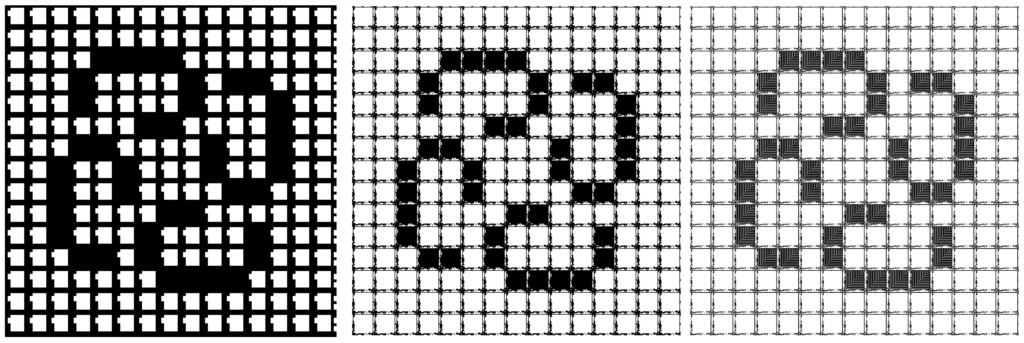
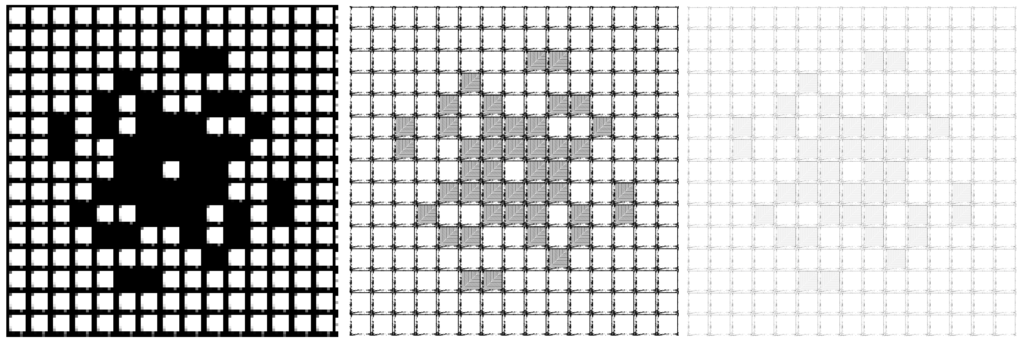
Figure x: Different resolutions for a 32768×32768 grid. On the top, the strategy of making the pixel as black or white based on the presence of a cell alive in the node. Basically, if the node that will represent a pixel has at least one cell alive, the whole node will represent a black pixel on the screen. Bellow, the strategy of making the brightness of the pixel be its area inverse. Hence, if the node have lots of live cells the screen pixel will be the darker.
From left to right, different depths thresholds giving rive to different resolutions to the final grid image.

There are some other minor language dependent technical issues but they are details. Other than that, we can keep the generation number (increasing based on the node size), skip empty nodes (not even cache then), etc.

Some results

Before I end this post (darn it, I can’t stop writing about this algorithm 😅) I would like to present some results and comment a bit about THE most interesting pattern in GoL (which is possible on because of the Hashlife algorithm).

Metacell

As Hashlife allows us to use big patterns into big grids, people started to invent all sorts of crazy patterns. There are patterns that spits gliders, pattens that “interact” with others to form new patterns, etc. There is even a way to “program” a pattern to do something. That can be done by using special smaller patterns that reacts to gliders when they hit it. Depending on the “state” of the pattern, it can perform action X or Y (produce another glider, or die, for example).

In 2006, a guy named Brice Due created a periodic 2048×2048 pattern called OTCA Metacell. It is a big square initially empty that looks like the next figure:

Figure x: OTCA Metacell. Source: LifeWiki

This is a programable pattern. Notice that when I say “programable” I don’t mean that we evolve it with different rules other than the 3 simple GoL rules. The grid still evolve using those 3 simple rules! What I mean by programable is that it has a special area with carefully crafted small patterns where you can “program” the behaviour of the whole grid by making the pattern evolve in a very specific way. When you start to evolve this Metacell, a small line of gliders starts to glide in the let side of the pattern in the direction of this “program area”. There, it hits some special patterns and, depending on the types of patterns that are present, it can “trigger” a chain reaction that turns “on” a set of glides guns in the top and right sides of the whole pattern. When those gliders generators activate, they start to produce gliders that “fills” up the entire empty region of the Metacell. Hence, we can say that this Metacell has two “states”. When the gliders guns are activated, the whole patterns fills up with gliders and it is “on”. When they are deactivated, we have the empty center region and the Metacell is considered “off”. The following animation shows a Metacell in the exact moment that it turning itself “on”.

The second most interesting aspect of this Metacell is that this “program area” communicates with inputs and outputs. There are 8 “inputs” that can sense external gliders and synchronise with the external world. Moreover, they are carefully designed to allow us to put two or more Metacells ones beside the others, allowing us to construct a “Metagrid” or Metagalaxy, as they call it. Now we can program the Metacell to turn itself on or off depending on the state of the neighbour Metacells. In fact, we can make a grid of Metacells behave like the the 3 GoL rules! Its the Game of life inside the Game of life!!!!!. In fact, the Wikipedia page about the Metapixel mention the work of guy named Adam P. Goucher that made a blinking MetaMetaCell (yes, 2 metas in the name). This means that we have a Metacell where each cell is itself o Metacell! I can’t help it to remember the Matrix movie… 😅 when I think of it.

It would be very difficult to construct or even to test such patterns if it wasn’t for the Hashlife algorithm. As an example, in the next section I’ll try to give some quantitative results for a Metacell. Just to put into perspective, one single Metacell has period of 35328 generations. That means that, in the regular GoL algorithm, we would have to evolve a 2048×2048 grid 35328 times to see only one step of the Metacell. Now imagine a grid 16×16 or even 64×64 Metacells…

Quantitative results

In this section I’ll try to show some results in terms of numbers. I’ll use a Metagalaxy composed of a 15×15 grid of Metacells. This makes up a 32768 x 32768 grid. In memory, the decompressed version of this grid would occupy 1073741824 bytes (~1GByte). The compressed array of nodes, with all the overhead like area of the nodes, depth, pointers to sub-nodes and etc, takes 1603559 Bytes (<2MBytes). The evolution time is slow in the beginning and gets faster as it evolves. Next figure shows a plot of the time to compute the generations, starting from the first one. It also shows the evolution of the cache size in bytes. As you can see, as the generations progress, the cache gets filled and, at some point stops growing (since this pattern is periodic).

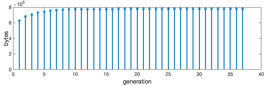
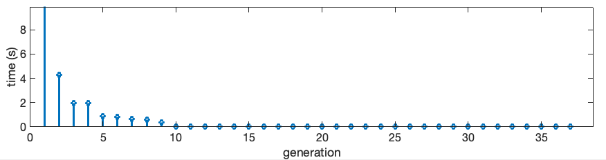
Figure x: Plots for time and memory consumption of the Metagalaxy example. The first generation takes around 50s to compute because the cache is getting filled (the Golly Java version does it in seconds, this 50s is my python implementation). But as soon as there is enough redundancy, the steps require less and less time, to the points that is practically instantaneous (even in Python).

Its worth to point out that “generations” here really means “steps” because remember that each step (which ends up taking milliseconds), actually computes generations at once (we pad 2 extra levels in the root node)!

If we turn on the “faster than light speed” and let the pattern evolve for 1min after the first generation (~2min total), we can evolve the pattern until the 1.152.921.504.606.781.440th generation!!! That’s 1 Quintillion generations!!! (I had to google the correct name hehehehe).

Finally I’ll leave you with the Metagalaxy evolution animation.

Figure x: Metagalaxy. It mimics the oscillator that we used as example in a 16×16 grid. The difference is that, in this one, each cell is a Metacell of size 2048×2048!

Conclusion

Hashlife is amazing! There is no other conclusion. It’s an amazing algorithm to solve an amazing problem. Period. Now I feel pushed to learn a bit about formal languages, automatons, and what not. I hope you enjoyed reading about Hashlife as much as I enjoyed writing about it (poor english and all %-). As always, the code is on GitHub if you want to look at it.
Thanks for reading!

References

Tomas G. Rokicki, blog post
Bill Gosper, original paper
jennyhasahat.github.io
Golly’s home page
Life Lexicon
Metapixel home page
Wikipedia entry