Introduction

In this post I’ll present another side project that I “had to do” during my participation in a project in Switzerland (as part of a pos-doc). I say “had to do” in quotes because, although was not one of my official attributions, it helped me A LOT to understand one of the main parts of the project and be able to develop the part I was responsible for.

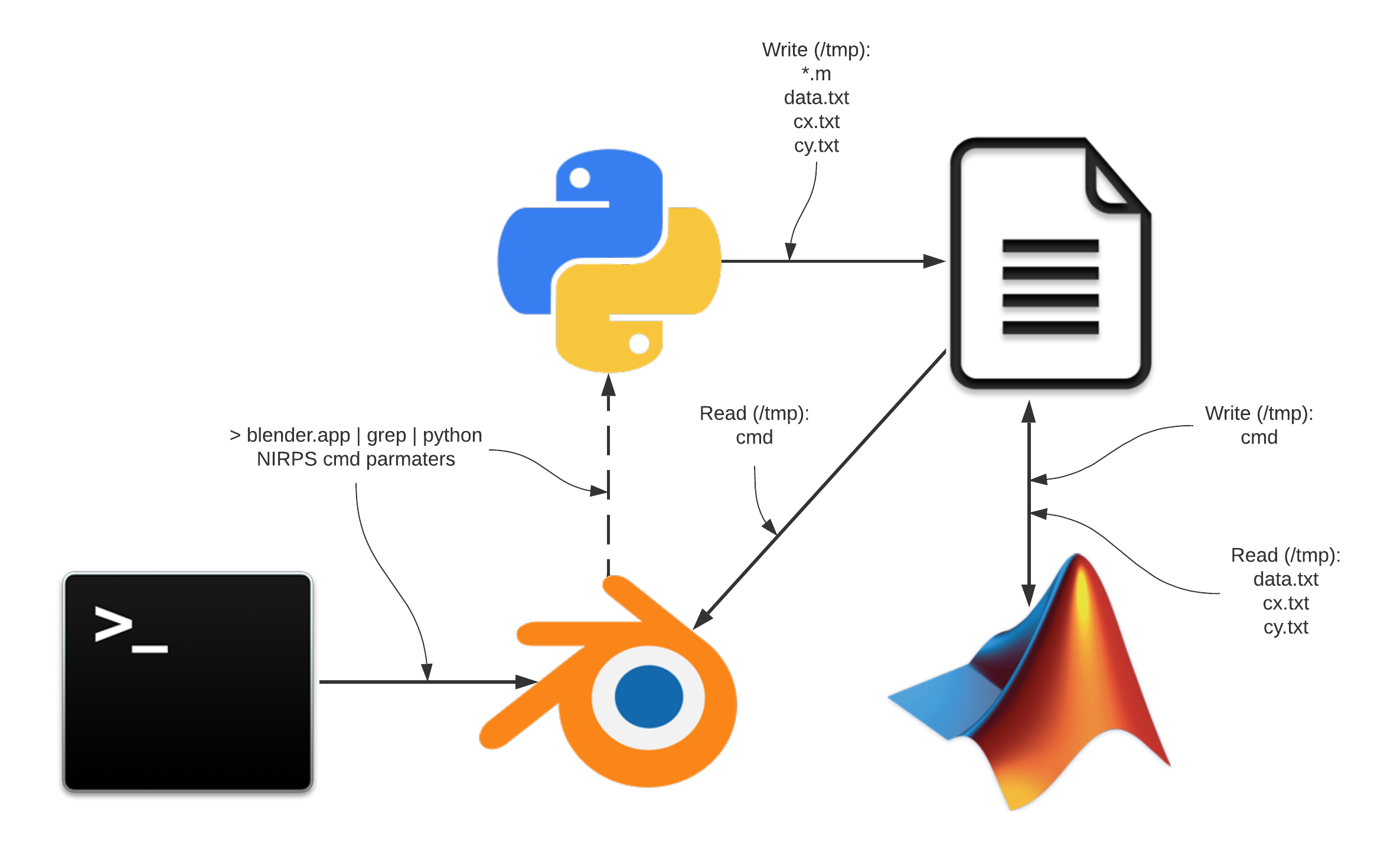
Briefly, the project is about the construction of a near infra-red spectrograph to be installed in a telescope in Chile. One of the novelties of this spectrograph is that it has an Adaptive Optics system to stabilise the images and optimize the performance of the instrument (details about the project in a future post). Hence, this post is about Adaptive Optics and more specifically, the small toy simulation I did in blender (together with C, python and Matlab) to understand how things work. In this post you will see no “blender” nor any implementation yet. Instead, I’ll talk about the theory behind it. In the next post I’ll talk about the implementation of the simulator itself.

Adaptive optics (just a tiny little bit)

general idea

Although the math and technology behind AO is extremely awesome and intricate, the basic idea of it is quite simple and the goal is straightforward. In short, the goal is to make the stars stop twinkle. The stars twinkle because of our atmosphere (see this post Wavefront sensing). In simple words, the atmosphere distorts the light that passes thought it randomly and thousands of times per second. That is what make its image “twinkle”. So, to simple put it, to make the stars stop twinkle, we have to un-distort the image of the star before it reaches the instrument (camera, spectrograph, etc). The way they do it is by deforming a flexible mirror with the “negative” of the distortion the atmosphere produces.

So, as you can see, the idea is straightforward. However, the amount of science and technology involved in doing it is breathtaking! First, we need to “measure” what is the deformation that the atmosphere is applying. Then, we have to apply that deformation (the negative of it) to a deformable mirror. Moreover, we have to do that thousands of times per second!!!
The animation bellow, tries to illustrate the process in a very very simplistic way. The first straight lines are the light coming from a star. The blue region is the atmosphere. When the lines passes through the atmosphere they start to “wiggle” to represent the distortion that the atmosphere introduces. The light bounces first into the deformable mirror (which is initially flat). Then it goes to a “splitter” that sends part of the light to the “sensor” that measures the deformation. The other part goes to a camera or instrument. The “sensor” sends the measurement to a computer that process it and computes the commands necessary to the deformable mirror. The deformable mirror then deforms and the light, from now on, becomes “straight”. Notice that, in the camera, the image of the star is “twinkling” at first. After the correction, the image becomes static and sharp.

<br />

Figure : Animation of an adaptive optics system

Thats the goal of an adaptive optics system. From that goal, comes a LOT of questions that have to be considered:

How to measure the deformation?
How to correct for that measured deformation?
How this correction can be computed?
Is this measurement noisy or precise? How to filter?
How to correct for the optics inside the instrument?
What kind of mathematical tools are needed?
and many more…

The goal of this project was exactly to try to answer/understand those questions.

The wavefront sensor

The wavefront sensor is the device that magically measures the deformation that the atmosphere is applying to the light that comes from the star. More impressively, its a camera (a special one, but an image device, nevertheless). That means that just by the light that arrives at the telescope, it can measure the deformation that was produced. Since this post is not about the device itself, for now its important to only understand what this measurement produces. For details on how a certain kind of wavefront sensor works, see Wavefront sensing)

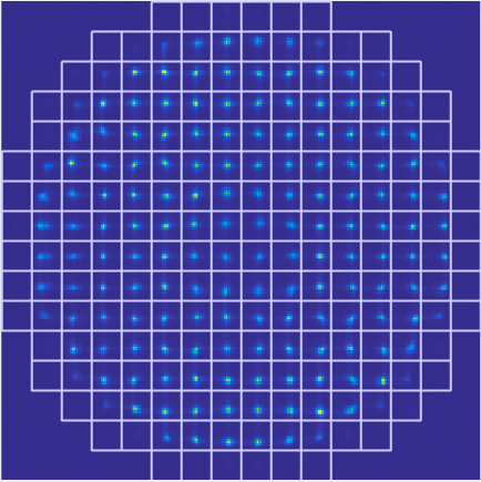
There are several types of wavefront sensors. The one we have in this simulation is called “Shack Hartmann wavefront sensor”. It works by imaging several “copies” of a point source light (the star) in different spacial positions in an CCD called “sub-apertures”. Depending on the spacial precision that we want to measure, we have more or less of those sub-apertures that produces the copies of the point light. By measuring the centroids of each sub image, it produces a “vector field” (called slopes) that corresponds to the direction and amplitude of the deformation at each place in space. The following figures shows a real measurement.

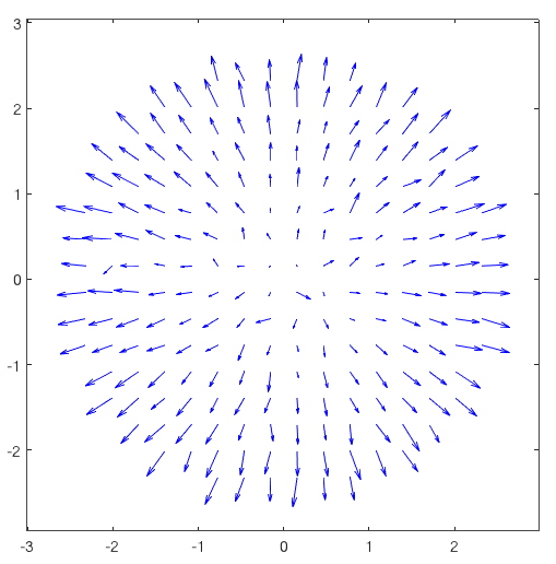Figure : First : Real image of a wavefront sensor (raw image, and marked sub-apertures marked). Second: Vector field resulting from a wavefront sensor measurement

The deformable mirror

As the name implies, this device is a mirror that has a deformable surface. As said before, the goal is to deform the light that comes from the atmosphere with the “negative” of its atmosphere deformation in order to make the effect of the atmosphere itself disappear.
The surface of this mirror is composed of several tiny actuators that pushes or pulls a point in the surface in order to deform it. As the wavefront sensor, depending on the precision we want to deform the light we can have from tenths to tenths of thousands actuators. Also, there are several types of actuators from piezoelectric to magnetic micro pistons.

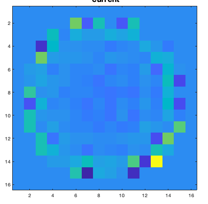
Figure : Sample of DM commands. Each “pixel” in this image represents the amplitude of an actuator. This image is what is sent to the mirror and its called “DM commands”.

Calibration (the Math behind it all)

In the following sections we will talk about the math behind an AO system. I’ll give the view of a non-AO engineer. In other words, I’ll not use the exact terms used in the area of adaptive optics. Instead, I’ll try to always see the AO processes (calibration, measurements, etc) as pure linear algebra operations. That is one of the beauties of using math to do physics 🙃.

The core of the math behind an AO system deals with two basic entities: the wavefront measurement and the commands applied to the DM. They form pair “input vs output” in the AO system. The main goal is to “map” the mirror commands $\mathbf{c}$ to wavefront slopes $\mathbf{s}$ in the sensor.
In practice, either the mirror and the wavefront slopes have a geometric “shape”. Because of that, we have to map the physical place of each actuator / slope. To do that, we define a “mask” for the mirror and for the WFS which contain the position of each element in the command vector

$\mathbf{c} = [c_1, c_2, ..., c_n]^t$

and in the slopes vector

$\mathbf{s} = [s_x_1, s_x_2, ..., s_x_m, s_y_1, s_y_2, ..., s_y_m]^t$

The figure bellow shows two examples of masks and the position os the elements of the command vector

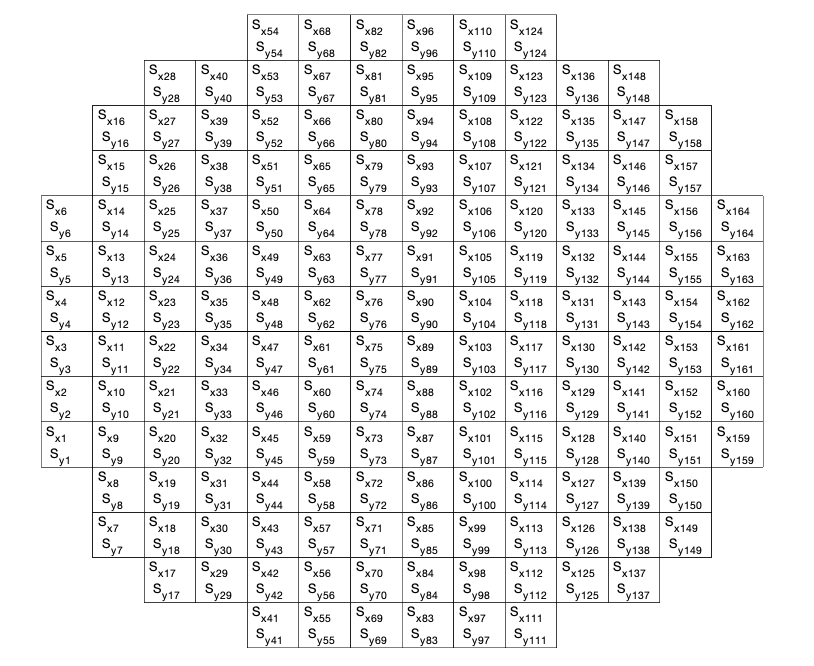
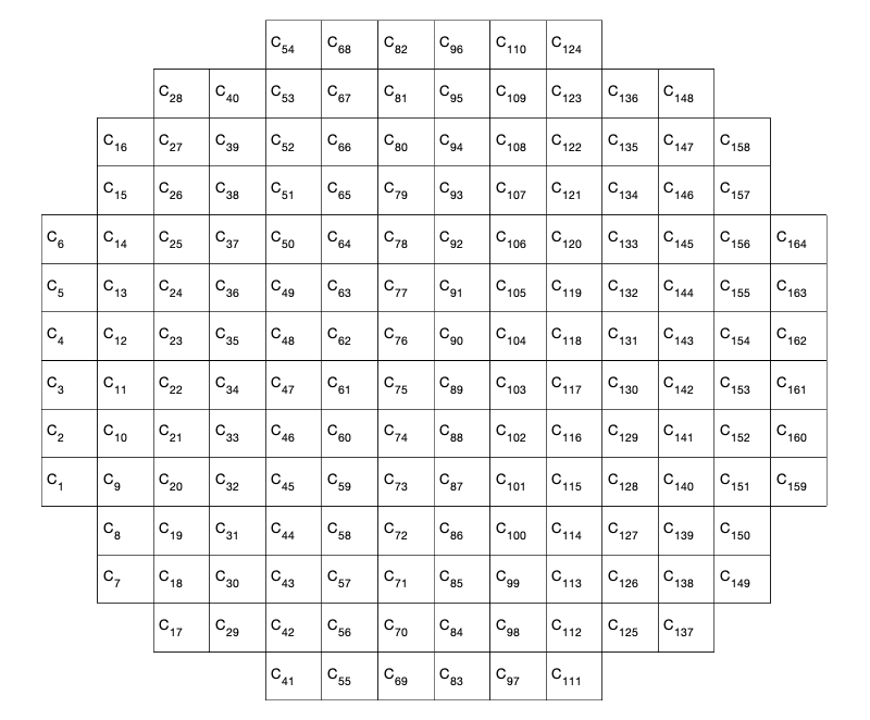
Figure: Example of masks defining the physical position of each command/slope in the actual devices

Using the laws of optics, in theory is possible to come up with the effect that the mirror will have on the light rays until reach the sensor and have a mapping $\mathbf{s} = f(\mathbf{c})$ . However, this function $f(.)$ is really complicated in general. It turns out that the slopes generated by the atmosphere are not so intense and a first order approximation for $f(.)$ is, in general, good enough. In fact, finding out this relationship is what they call “calibration”.

Interaction matrix

In principle (and theoretically) the function $f(.)$ should behave as a discrete differentiation. In other words, a plane wave driving to the mirror should take the form of the commands and the WFS would measure the local slopes of the wavefront. That is exactly what a differentiation would do. However, the differences in size between WFS and the mirror, factors like crosstalk between actuators and etc forces us to “calibrate” and find a suitable mapping $f(.)$ which is exclusive to the pair Mirror / Sensor we have.

The first order approximation for the function $f(.)$ represents a linear mapping between mirror commands and wavefront slopes and can be written as

$\mathbf{s} = \mathbf{M}\mathbf{c}$

where $M$ is called interaction matrix. Interaction matrix is a matrix whose columns corresponds to the slopes on the WFS and each line corresponds to an actuator of the DM. The value is the local light displacement in the WFS subaperture (x for the first half of the columns and y for the second half of the columns).

Here is where the math starts. Now, the whole of adaptive optics boils down to the study, process and understanding of a linear space defined by the relation of the equation above.

To obtain this matrix we have to sample several slopes $\mathbf{s}$ from several commands $\mathbf{c}$ . In theory, we could just randomly command the mirror, measure the slopes and find out $\mathbf{M}$ . However, since we have full control of what we command, we just can push each actuator of the mirror letting all the other in zero position. If we stack side by side each command for an individual actuator, we will end up with an identity matrix for the vectors $\mathbf{s}$ and a set of row measurements for the vectors $\mathbf{s}$ . Hence we have a stack of measurements

$\mathbf{S} = [\mathbf{s}^{(1)}, \mathbf{s}^{(2)}, \mathbf{s}^{(3)}, ..., \mathbf{s}^{(N)}]$

and

$\mathbf{C} = [\mathbf{c}^{(1)}, \mathbf{c}^{(2)}, \mathbf{c}^{(3)}, ..., \mathbf{c}^{(N)}]$

where $\mathbf{s}^{(i)}$ and $\mathbf{c}^{(i)}$ are the measured slopes and command for the sample $i$ . In particular, $\mathbf{c}^{(i)} = [0, 0, 0, ..., 0, 1, 0, ..., , 0, 0]$ making $\mathbf{S} = \mathbf{I}$ (the identity matrix).

Although there are several ways to sample the interaction matrix space, this one is interesting because now the relationship becomes $\mathbf{s} = \mathbf{M}\,\math{I} = \mathbf{M}$ . In other words, the measurements themselves assemble the interaction matrix. Those measurements are done sequentially and the animation bellow illustrates the procedure.

Figure : Animation of the pinch procedure for calibration. In the left we have the slopes and in the right we have their amplitudes.

After all measurements, the interaction matrix is ready to be used in the AO system. Of course that, in practice, some technical and practical aspects are different. For instance, they push and pull the actuators more than one time, or use another set of samples commands, like a Hadamard shaped command. For the purpose of this simulator, the identity was enough. Bellow we have an example of an interaction matrix resulting form this procedure.

Figure : Interaction matrix example

With the interaction matrix at hand, we now can do the optical “analysis”. In other words, we can predict what the slopes $\mathbf{s}$ will be if we deform the mirror with a particular shape using commands $\mathbf{c}$ . But this is not what we want. In fact we want the exact opposite. We want to measure the atmosphere shape and deform the mirror such as to produce the negative of the measured shapes. Since we have a linear relationship, this seems easy enough. We just invert the interaction matrix and write $\mathbf{c}$ as a function of $\mathbf{s}$ right? Not so fast… First of all, $\mathbf{M}$ is not square. That immediately tell us that there are more degrees of freedom in the commands $\mathbf{c}$ . Which mean that for the same slopes $\mathbf{s}$ , there might be an infinite number of commands that have those slopes as a result. Because of that, we have a whole lot of math to help us choose the right commands to apply to the mirror. This is what we will explore in the next sections.

Phase decomposition

Now that we boiled down the whole AO business to a linear relationship, we can do a lot of tricks with it. Probably the most important thing we should do is to analyse the structure of the matrix $M$ . This matrix embeds the whole optics of command vs slopes in its values. For this kind of analysis, it is really helpful to visualise the linear relationship as blocks of vectors as described by the following figure.

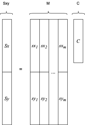
Figure : Linear relationship as combinations of columns of $\mathbf{M}$

Here, we see that the slopes are organised as X and Y in a vector and that the column space of $\mathbf{M}$ spans its space. In other words, the final slopes are a linear combination of some other more basic slopes and the combination is exactly the commands $\mathbf{c}$ .

Now lets then decompose $\mathbf{M}$ in its singular values and write

$\mathbf{M} = \mathbf{V}\mathbf{D}\mathbf{U}^t$

In this decomposition, the column space of $\mathbf{M}$ is rewritten or projected in another basis $\mathbf{V} = [\mathbf{v}_{0,1},\mathbf{v}_{0,2},...,\mathbf{v}_{0,n}]$ which is orthonormal. Each $i^{th}$ column of $\mathbf{U} = [\mathbf{u}_{0,1},\mathbf{u}_{0,2},...,\mathbf{v}_{0,m}]$ together with its corresponding $\mathbf{D} = diag(d1,d_2,d_3,...,d_m,0,0,...0)$ is the coordinate of the $i^{th}$ column of the original matrix $\mathbf{M}$ . This relationship is illustrated in the diagram bellow

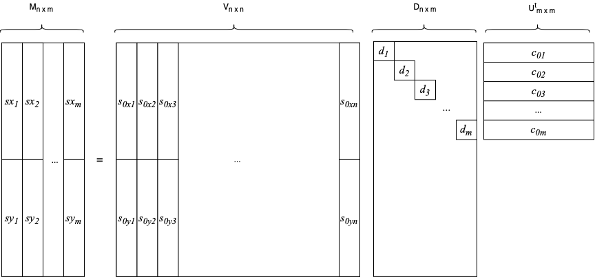
Figure : Block representation of the decomposition of $\mathbf{M}$

With this representation in mind, we can analyse a little bit further what are the projected vectors $\mathbf{v}_{0,i}$ and the vectors $\mathbf{u}_{0,j}$ . By the construction of the decomposition, $\mathbf{v}_{0,i}$ is an orthonormal projected version of the columns of $\mathbf{M}$ which means that they are slopes. Since $\mathbf{v}_{0,i}$ are coordinates (weights for the combination of the slopes $\mathbf{v}_{0,i}$ ), they are commands.

Now the question is: What are those “special” set of slopes and commands?

Modes

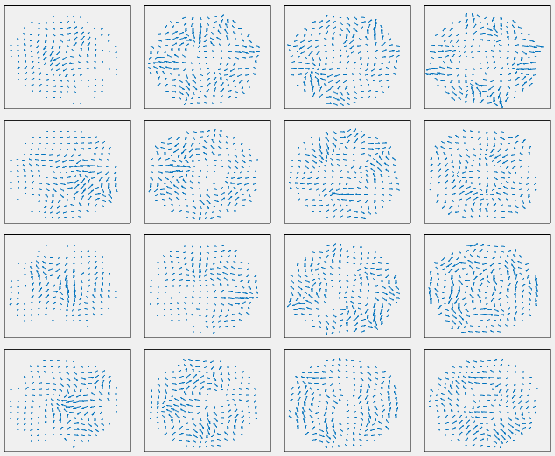
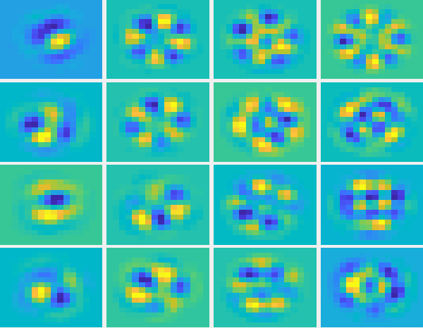
The answer to the previous question is: Despite the fact that the “special” commands and slopes are orthogonal among themselves, there is nothing optically special about them. They are called “modes”. The figure bellow shows a typical set os modes for commands and slopes from an adaptive optic system.

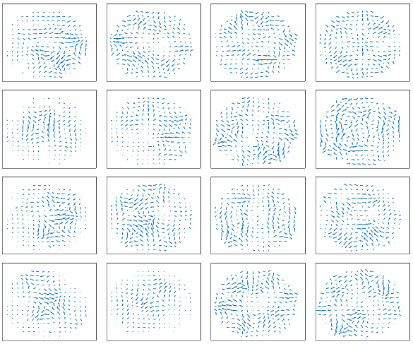
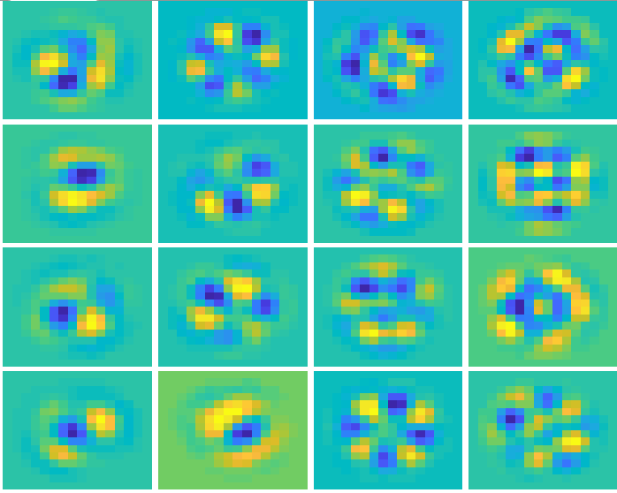Figure: Slopes and commands modes. Result of the SVD decomposition of the interaction matrix.

The relationship between each command mode and the slopes mode is quite straightforward. If we compute the slopes $\mathbf{s}$ for any given special command, say $\mathbf{u}_{0,i}$ we have

$\mathbf{s} = \mathbf{M}\,\mathbf{u}_{0,i}$

$\mathbf{s} = \mathbf{V}\,\mathbf{D}\,\mathbf{U}\,\mathbf{u}_{0,i}$

Since all the rows of $\mathbf{U}$ are orthogonal to each other and $\mathbf{u}_{0,i}$ is one of those rows, the last term ( $\mathbf{U}\,\mathbf{u}_{0,i}$ ) will be basically a vector with zeros everywhere except on the i’th row. When we multiply this vector with $\mathbf{D}$ we basically “select” the $d_i$ and now we have a vector with zeros except for $d_i$ in the i’th row. Multiplying now this vector by $\mathbf{V}$ means that we select the i’th column of $\mathbf{V}$ multiplied by it corresponding $d_i$ . In short, when we apply one of the command modes, we end up with the corresponding slopes mode. By the way, those modes are called “zonal” modes and they are the ones that comes out of the SVD decomposition of the interaction matrix.

Now we can focus on the generic commands we will send to correct for the atmosphere. Since those commands will come from the interaction matrix (its inverse, to be more precise) it will be a linear combination of the basis we got in the SVD decomposition. Since that basis is an orthonormal basis, we can easily decompose back the command into its components in this “zonal modes”.

The question is, why decompose back? We mentioned before that when we use one of the modes as commands, we “select” the corresponding mode in the slopes weighted by the corresponding eigenvalue $d_i$ . If look at the distribution of the eigenvalues, we notice that they decrease in amplitude up to values that are very small (See next figure).

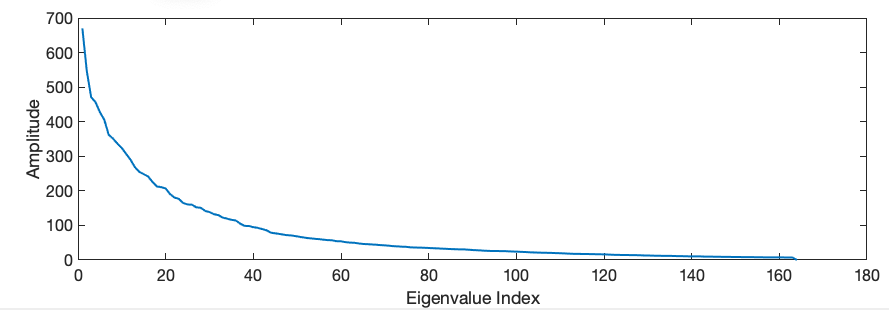
Figure: Distribution of the eigenvalues in the interaction matrix SVD decomposition

if we are solving the inverse problem, we will present a set of slopes and we will produce the commands necessary to generate those slopes. If that particular set of slopes had a mode corresponding to a small eigenvector, we will need a very high amplitude in the respective command to generate it. That will produce a mirror configuration with a crazy shape because remember that all we are doing depend on small displacements for the mirror. But those slopes might occur due to measurement noise, small optical artifacts, etc. So the solution is to decompose the generated commands and “filter” out those crazy modes.
Hence, the procedure is: We decompose, eliminate the crazy ones, and “recompose” back the commands. When we apply this new command, we won’t have the original desired slopes, but a “smoother” version of it which probably will be fine.

KL modes

We can look at the problem of finding the interaction matrix as a “regression” problem. We have a linear relationship that we want to find and have some samples of it. That linear relationship defines a space. When we do the poking of the mirror each actuator at a time, we are “sampling” the space in order to compute that linear relationship. In that sense, the zonal modes are a new basis for this space. However, there are infinitely many basis. In that sense, we could try to find a new basis that might have a statistical significance or interpretation. One in particular that might be useful is the Karhunen–Loève basis or KL for short. The KL basis is obtained by taking the eigenvectors of the covariance matrix of the samples. This is the procedure used in several techniques like principal component analysis (PCA). The idea is that the covariance matrix defines an ellipsoid in the sample space. In that ellipsoid (in several dimensions, or course) each axis is an eigenvector and its length is the associated eigenvalue. The advantage of this new basis is that each eigenvalue represents the variance of the sampling in that particular direction (or mode). Hence, small eigenvalues might mean that, the corresponding eigenvalue / mode, is just “noise” and could be thrown out or ignored.
The next figure shows some of the KL modes, just as an illustration.

Figure: Slopes and commands for the KL modes.

Visually the modes are not so different than the zonal ones. They all have the “humps” and “valleys” which are normal for matrices with the geometry of the interaction matrix. However, if we loop at the distribution of the modes in termos of its corresponding eigenvalues, we see a big difference (see next figure). In the KL version, we have a lot more small eigenvalues, meaning that we can consider reconstructions with less modes having the same overall loss in information.

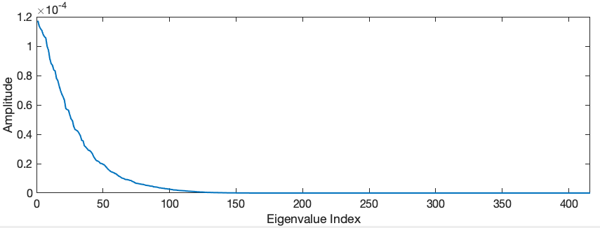
Figure: Distribution of the eigenvalues in the interaction matrix KL decomposition

Zernike modes

Up to this point, a lot of the math sophistication in an adaptive optics system boils down to choose a good set of modes which, in turn means to select a good basis where we can project the commands onto. Hence, yet another interesting basis that could be used is called Zernike Basis. This basis is based on a special set of polynomials called Zernike Polynomials. It deserves an entire post only for it but, in summary, its a set of ortogonal polynomials defined in the unity circle. Each polynomial in this set is characterised by two numbers $(m,n), m > n$ that defines the degree of the polynomial. The following figure shows a plot for some of those polynomials.

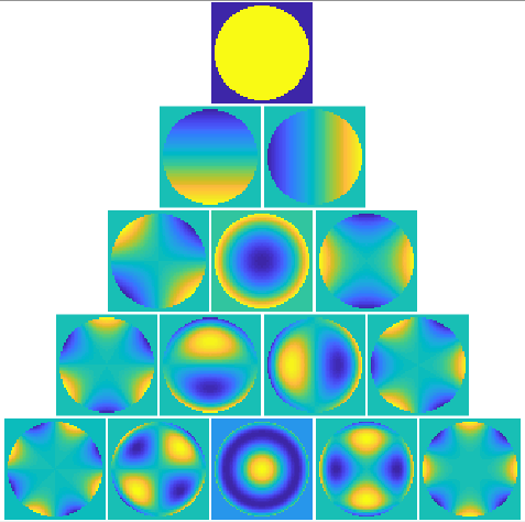
Figure: Plot for $Z_{0,0}(x,y), Z_{1,0}(x,y), Z_{1,1}(x,y), Z_{2,1}(x,y), ...$

It turns out that those “Zernike modes” are optically meaningful! First they have nothing to do specifically with AO. They are very useful in optics in general. For instance eye doctors refer to them a lot to describe eye defects. The first one even have familiar names to us like Astigmatism, Coma and Defocus.

But the Zernike polynomials are polynomials. To be used as a basis in AO they need to be spatially sampled to be the size of the DM (and hence be used as commands). However, we need to be cautious because after spatially sampled, the resulting discrete set (command to be applied in the DM) is not orthogonal. Nevertheless, the main use of Zernike modes are not to work as a basis per se, but instead to be “applied” to the system and measure the result.

The point Spread Function

When we finally have the right modes, filtering and etc, the light ends up arriving to the camera and/or detector. An interesting question is: What should we expect to see if the system do its job well? We should see the perfect image of the star, right? Well, unfortunately no… First of all, in general, the star is really really tiny and “a perfect image of a star” would be few pixels with a high brightness and all the other pixels with zeros or very low brightness. That would be very good if it happened, but there is a physical (optical) limitation: the aperture of the telescope.

The image that we expect to see, the little “dot” representing the star, is called point spread function or PSF in short. As mentioned in the paragraph above, even if everything is perfect and a completely plane wave reaches the telescope its finite aperture, combined with the “shadow” of the secondary mirror have an effect in the image. It turns out that the image we see is the the inverse Fourier transform of the “image” in the pupil of the telescope. “Image” is in quotation in the previous sentence because it’s not an image per se. Instead it is an image where we have constant amplitude where the light goes through and the phase modulated by the slopes of the light that arrives. If the wave is perfectly plane we have a constant amplitude there the light goes though and a constant phase. In this case, the image that is formed in the detector/camera is not a perfect point (as the object truly is) but instead, a smoothed point with little rings around it. The next figure shows an example.

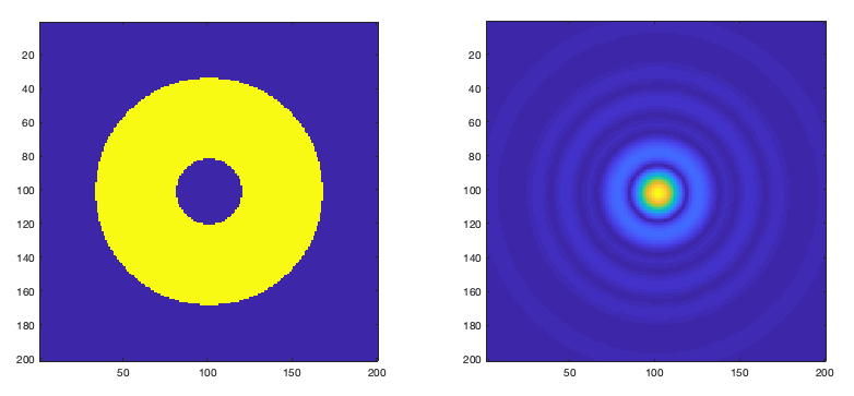
Figure: Example of a pupil “image” and its corresponding camera image. We see, in the pupil, the area where the light enters and the shadow of the secondary mirror in the middle. In the camera we see the PSF which is not a perfect point.

The explanation for this Fourier relationship between the pupil and the PSF image is, in on itself, a huge topic called Fourier Optics. That deserves a post (or more) by itself. There is another important relationship we gather from the area of Fourier Optics. If the image that we are observing is not a point, let say a planet, we can predict what it will show up in the camera. It turns out that it’s the convolution of the PSF with the original clear image. That is why there is a limit of how clear an image can be imaged even if we had no atmosphere at all!

Now we might ask the question: What happens if the phase that arrive is not constant, but modulated by the atmosphere? To have an idea of what happens, we can take a look at the distortions caused by the modes themselves (in particular the Zernikes since they have optical use). The next figure shows the PSFs for each Zernike. Each one is the result PSF for a system with circular aperture (like an eye or a telescope with no secondary mirror) and phase modulated by the Zernike shape. As mentioned before, each shape have a name in Optics like “Astigmatism”. In fact when a person suffers from Astigmatism, it means that the “lenses” formed by the eye have that Zernike shape! So, to emulate what a person with astigmatism sees, we convolve the astigmatism PSF with the image and voila! You can have an idea what is like to have the problem.

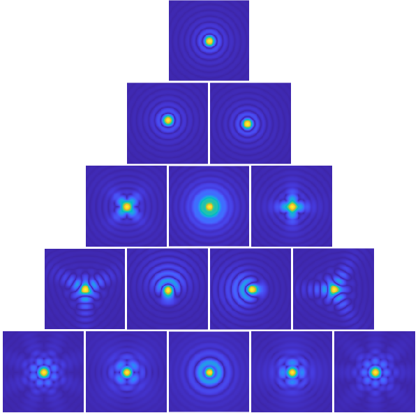
Figure: Set of PSFs for each corresponding Zernike mode

In particular, the 2nd and 3rd Zernike are called “Tip” and “Tilt”. If you look at the corresponding PSFs, we notice that they don’t change shape. Instead, they “displace” the PSF to the right or to the left (Tip) and up or down (Tilt). Hence, they are the responsible for the movement of the star in the camera. Wen we see the start twinkling and moving around, the moving around is the result of the optical mode Tip and Tilt combined together.

NCPA

Another common calibration that is needed in an AO system is called Non-Common Path Aberration (NCPA). It deals with the fact that optical elements in the system might introduce optical distortions or aberrations. One might argue that, since we measure the distortions with the WFS, why to calibrate for the optics of the system? Shouldn’t the calibration of the interaction matrix take that into consideration too? The answer is yes, but for the light path until the WFS! If we look at the first figure with the small animation in the beginning of this post we see that, at some point, the light splits from the DM to the WFS and Camera/Detector. Everything in the path to the camera is not sensed by the WFS, thus not corrected by the DM. So, they are aberrations that are not common to the path of the WFS (hence the name, NCPA).

But how do we correct for those aberrations that are not sensed by the WFS? In another words, how do we measure those aberrations in order do eliminate them? The answer is, we don’t! There is a very clever trick the engineers came up with that involves using the previous calibration (the interaction Matrix) to help. To correct for the the NCPA, we assume that the interaction Matrix is calibrated. That means that we can produce any shape on the DM accurately. Hence, the AO system have a special light source (normally a Laser) that is placed before the mirror and simulates a perfect point source of light. With that light, if the mirror is flat, we should see the PSF corresponding to the shape of the mirror and the optics in the path (in general circular). Due to the NCPA, the image will not be a perfect PSF, but instead, a distorted version of it.

The trick to figure out the distortion is to try to “guess” the distortion. A very very naive was to do that is to search several mirror configurations until one of them makes a perfect PSF that look like a pane wave PSF in the camera (the WFS is already calibrated). Of course that this is nonsense due to the infinite number of possibilities. Fortunately, we don’t need to test randomly. We could use certain configurations where we know what to expect in the image. Those are exactly the Zernike modes.

Hence, the NCPA algorithm is pretty simple. We apply each Zernike mode skipping the first one which is flat and also the Tip and Tilt which does not change the shape of the PSF. We apply them to the DM sequentially scanning the amplitude from, say, -0.5 to 0.5 and observe the image. The one which looks more like the mode we know we store the amplitude we are applying and that would be the current amplitude for that mode that corrects the NCPA. We do that for several modes (say the first 10 or 30). In the end we will have for each Zernike mode, a small amplitude that, together, corrects the NCPA. Unfortunately when we are correcting for one mode we might slightly de-correct for the previous, that’s why we have to do several iterations of this sequence. In a sense, we are solving an optimisation problem by looking in each dimension at a time interactively.

In summary, we have to find a vector $\mathbf{a}=\left[a_1, a_2, a_3, ..., a_N\right]$ of amplitudes for the fist $N$ Zernike modes which, when applied together to the DM, will make a perfectly flat PSF (just the small blob with the rings). The algorithm here will search for the point in the Nth dimensional hyper volume defined by setting limits for each amplitude like $-A_i < a_i < A_i<$ . In the end the command that corrects the NCPA would be

$\mathbf{c}_{NCPA} = \sum_{i=1}^{N}a_i\,\mathbf{z}_i$

where $\mathbf{z}_i$ are the Zernike modes. Fortunately, the “function” we are optimising is convex and can be easily tested by measuring the flux of the brightest pixel in the image. Hence, we are optimising the maximum flux possible in a pixel of the camera image.

The algorithm is shown in the next figure. There, $N_i$ is the number of iterations. $N_z$ is the number of Zernike modes to search. $A$ is the maximum amplitude for the Zernike amplitudes. $N_a$ the number of amplitudes to scan from $-A$ to $A$ .

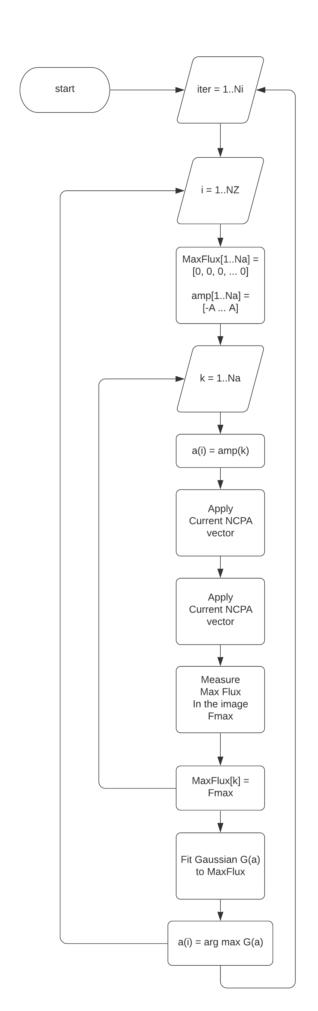
Figure: NCPA algorithm

One interesting point in the algorithm is that each measurement is not instantaneous, so if we have, say, 4 iterations, for 30 Zernikes we will have to scan 120 times. In order to find a good optimisation we have to have a “fine” scan for each Zernike. The engineers try to narrow down as much as possible the limits in the amplitudes (value of $A$ ) but we still have to look for several values in this range. Say that we have $A = 0.5$ hence, we scan from -0.5 to 0.5. Which step should we use? If we want a fine search we have to subdivide to get a 0.001 precision, we would have to compute 100 steps. That would have to be done for each of the 120 iterations/Zernikes. Clearly, that is too much. Instead, the trick is simple. We do very few steps (like 5 or 7) and fit a curve over the points (a Gaussian, for instance). Then we compute its maximum analytically. The next animation shows a real PSF resulting from the execution of an NCPA algorithm.

Figure: Animation of the PSF in a real NCPA execution during NIRPS development

Another technical aspect that the NCPA algorithm can help is when we don’t have a mirror that can be made “flat” via command. Some Mirrors have piezo actuators and we do not control exactly their position. Se send each actuator to a position but we have no feedback wether it is in he right place. This kind of mirror is very difficult to be made “flat”. With the help of NCPA algorithm we can correct for that actuator error also. The next figure shows a plot of a real NCPA result. Each line in the plot is a Zernike / iteration. The fitted Gaussian can also be seeing for each mode.

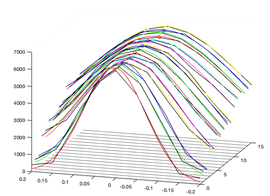
Figure: Example os real measurements in an NCPA performed on the NIRPS instrument

To be continued…

In the next post we see the part II of this big post/project

References

Adaptive Optics – https://en.wikipedia.org/wiki/Adaptive_optics
SVD – https://en.wikipedia.org/wiki/Singular_value_decomposition
KL Transform – https://en.wikipedia.org/wiki/Karhunen–Loève_theorem
Zernike Polynomials – https://en.wikipedia.org/wiki/Zernike_polynomials
Fourier Optics – https://en.wikipedia.org/wiki/Fourier_optics
New concepts for calibrating non-common path aberrations in adaptive optics and coronagraph systems – https://arxiv.org/pdf/1909.05224.pdf

3 thoughts on “Using Blender to learn the basics of Adaptive Optics (part I / II)”

Leslie

March 15, 2023 at 8:16 am

How did you build the optical elements?
In Blender or other tool and then you import them to Blender?
Are you using any special light rendering engine in Blender? or Cycles?
I am interested in implementing an optical system in Blender and simulate it.
Thank you for any suggestion.

- ninguem
  
  March 15, 2023 at 9:49 am
  
  Hello!
  Thank you for the comment! Take a look into the part II of this post, there I explain the general idea of the implementation and also give the link for the GitHub with the code! (search for blender adaptive optics on GitHub)
  
Leslie

March 15, 2023 at 8:16 am

How did you build the optical elements?
In Blender or other tool and then you import them to Blender?
Are you using any special light rendering engine in Blender? or Cycles?
I am interested in implementing an optical system in Blender and simulate it.
Thank you for any suggestion.
Leslie