Introduction
Wavefront sensing is the act of sensing a wave front. As useless as this sentence gets, it is true and we perform this action with a wavefronts sensor… But if you bare with me, I promise that its going to be one of the coolest mix of science and technology that you will hear about! Actually, I promise that it would be even poetic, since that, in this post, you will learn why the stars twinkle in the sky!
Just a little disclaim before I start: Im not an optical engineer and I understand very little about the subject. This post is just myself sharing my enthusiasm about this amazing subject.
Well, first of all, the word sensing just mean “measure”. Hence, wavefront sensing is the act of measure a wave front with a wavefront sensor. To understand what a wavefront measurement is, let me explain what a wavefront is and why one would want to measure it. It has to do with light. In a way, wavefront measurement is the closest we can get from measuring the “shape” of a light wave. The first time I came across this concept (here in the Geneva observatory) I asked myself: “What does that mean? Doesn’t light has the form of its source??”. I guess thats a fair question. In the technical use of the term measurement, we consider here that we want to measure the “shape” of the wave front that was originated in a point source of light very far away. You may say: “But thats just a plain wave!” and you would be right if we were in a complete homogeneous environment. If that were the case, we would have nothing to measure %-). So, what happens when we are in a non-homogenous medium? The answer is: The wavefront gets distorted, and we got to measure how distorted it is! When light propagates as a plain wave and it passes through an non-homogeneous medium, part of its wavefront slows down and others don’t. That creates a “shape” in the phase of the wavefront. Because of the difference in the index of refraction of the medium, in some locations, the oscillation of the electromagnetic arrives a bit earlier and some other it arrives a bit later. This creates a diferente in phase at each point in space. The following animation tries to convey this idea.

Figure 1: Wavefront distorted by a medium
As we see in the animation, the wavefront is plain before reaching the non-homogeneous medium (middle part). As it passes through the medium, it exits with a distorted wavefront. Since the wavefront is always traveling in a certain direction, we are only interested in measure it in a plane (in the case of the animation, a line) perpendicular to its direction of propagation.
In the animation above, a measurement at the left side would result in a constant value since, for all “y” values of the figure, the wave arrives at the same time. If we measure at the left side we get something like this
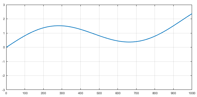
Figure 2: Wavefront measurement for the medium showed in Figure 1
Of course that, in a real wavefront, the measurement would be 2D (so the plot would be a surface plot).
An obvious question at this point is: Why someone would want to measure a wavefront? There is a lot os applications in optics that requires the measurement of a wavefront. For instance, lens manufacturer would like to know if the shape of the lenses they manufactured is within a certain specification. So they shoot a plane wavefront through the lens of the glass and measure the deformation in the wavefront causes by the lens. By doing that, they measure the lens properties like astigmatism, coma and etc. Actually, did you ever asked yourself where those names (defocus, astigmatism, coma) came from? Nevertheless, one of the the most direct use of this wavefront measuring is in astronomy! Astronomers like to look at the stars. But the stars are very far away and, for us, they are an almost perfect point source of light. That means that we should receive a plain wave here right? Well if we did we have nothing to breath! Yes, the atmosphere is the worst enemy of the astronomers (thats why they spend millions and millions to put a telescope in orbit). When the light of the star or any object passes through the atmosphere, it gets distorted. Its wavefront make the objet’s image swirl and stretch randomly. Worst then that, the atmosphere is always changing its density due to things like wind, clouds and difference in temperatures. So, the wavefront follows this zigzags and THAT is why the stars twinkle in the sky! (I promise didn’t I? 😃) So, the astronomers build sophisticated mechanisms using adaptive optics to compensate for this twinkling and that involves, first of all, to measure the distortion of the wavefront.
Wavefront measurement
So, how the heck do we measure this wavefront? We could try to put small light sensors in an array and “sense” the electromagnetic waves that arrives at them… But light is pretty fast. It would be very very difficult to measure the time difference between the rival of the light in one sensor compared to the other (the animation in figure 1 is like a SUPER MEGA slow motion version of the reality). So, we have to be clever and appeal to the “jump of the cat” (expression we use in Brazil to mean a very smart move to solve a problem).
In fact, the solution is very clever! Although there are different kinds of wavefront sensors, the one I will explain here is called Shack–Hartmann wavefront sensor. The ideia is amazingly simple. Instead of measuring directly the phase of the wave (that would be difficult because light travels too fast) we could measure the “inclination” or the local direction of propagation of the wavefront. Now, instead of an array of light sensors that would try to measure the arrival time, we make an array of sensors that measure the local direction of the wavefront. With this information it is possible to recover the phase of the wavefront, but that is a technical detail. So, in summary, we only need to measure the angles of arrival of the wavefront. Figure 3 tries to exemplify that I mean:

Figure 3: Exemple of measurement of direction of arrival, instead of time of arrival.
Each horizontal division in the figure is a “sub-aperture” where we measure the inclination of the wavefront. Basically we measure the angle of arrival, instead of the time of arrival (or phase of arrival). If we do those sub-apertures small enough, we can reconstruct a good picture of the wavefront. Remember that for real wavefronts we have a plane, so we should measure TWO angles of arrival for each sub-aperture (the angle in x and the angle in y, considering that z is the direction of propagation).
At this point you might be thinking: “Wait… you just exchanged 6 for 12/2! How the heck do we measure this angle of arrival? It seems that this is far more difficult then to measure the phase itself!”. Now its time to get clever! The idea is to put a small camera in each sub aperture. Each tiny camera will be equipped with a tiny little lens to focus the portion of the wavefront to a certain pixel of this tiny camera! Doing that, at each camera, depending on the angle of arrival, the lens will focus the locally plain wave to a certain region of the camera dependent on the direction its traveling. That will make each camera see a small region with bright pixels. If we measure where those pixels are in relation to the center of the tiny camera, we have the angle of arrival!!! You might be thinking that its crazy to manufacture small cameras and small lenses in a reasonable packing. Actually, what happens is that we just have the tiny lenses in front of a big CCD. And it turns out that we don’t need hight resolution cameras in each sub-aperture. A typical wavefront sensor has 32×32 sub apertures, each one with a 16×16 grid os pixels. That is enough to give a very good estimation of the wavefront. Figure 4 shows a real image of a wavefront sensor.
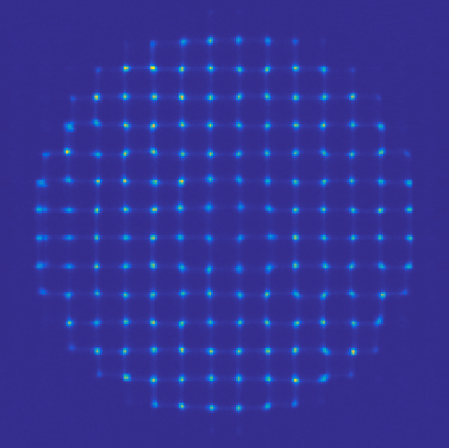
Figure 4: Sample image from a real wavefront sensor
Simulations!
The principle is so simple that we can simulate it in several different ways. The first one is using the “light ray approach” for optics. This principle is the one we learn in college. Its the famous one that they put a stick figure on one side of a lens or a mirror and them draw some lines representing the light path. The wavefront sensor would be a bit more complex to draw, so we use the computer. Basically what I did was to make a simple blender file that contains a light source, something for the light to pass through (atmosphere) and the sensor itself. The sensor is just an 2D array of small lenses (each one made up by two spheres intersected) and a set of planes behind each lens to receive the light. We then set up a camera between the lenses and the planes to be able to render the array of planes, as they would be the CCD detectors of the wavefront sensor. Now we have to set the material for each object. The “detectors” must be something opaque so we could see the light focusing on it. The atmosphere have to be some kind of glass (with a relatively low index of refraction). The lenses also have glass as its material, but their index of refraction must be carefully adjusted so the focus of each one can be exactly on the detectors plane. Thats pretty much it (see figure 5).
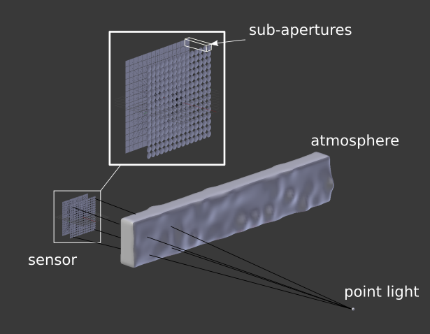
Figure 5: Setup for simulating a wavefront sensor in blender
To simulate the action, we move the “atmosphere” object back and forth and render each step. As light passes through the object, it diffracts it. That changes the direction of the light rays and simulates the wavefront being deformed. The result is showed in figure 6.
Figure 6: Render of the image on the wavefront sensor as we move the atmosphere simulating the real time reformation of the wavefront.
Another way of simulating the wavefront sensor is to simulate the light wave itself passing through different mediums, including the leses themselves and driving at some absorbing material (to emulate the detectors). That sounds kind of hardcore simulation stuff, and it kind of is. But, as I said in the “about” of this blog, I’m curious and hyperactive, so here we go: Maxwells equations simulation of a 1D wavefront sensor. To do that simulation, I used a code that I did a couple of yeas back. I’ll make a post about it some day. It is an implementation of a FD-TD (Finite Diferences in the Time Domain) method. This is a numerical method to solve partial differential equations. Basically, you set up your environment as a 2D grid with sources of electromagnetic field, material of each element on the grid and etc. Then, you run the interactive method to see the electromagnetic fields propagating. Anyway, I put some layers of conductive material to contain the wave is some points and to emulate the detector. Then I added a layer with small lenses with the right refraction index to emulate the sub-apartures. Finally, I put a monochromatic sinusoidal source in one place and pressed run. Voilá! You can see the result in the video bellow.
The video contains the explanation of each element and, as you can see, the idea of a wavefront sensor is so brilliantly simple that we can simulate it at the Maxwells equation level!
DIY (physical) experiment
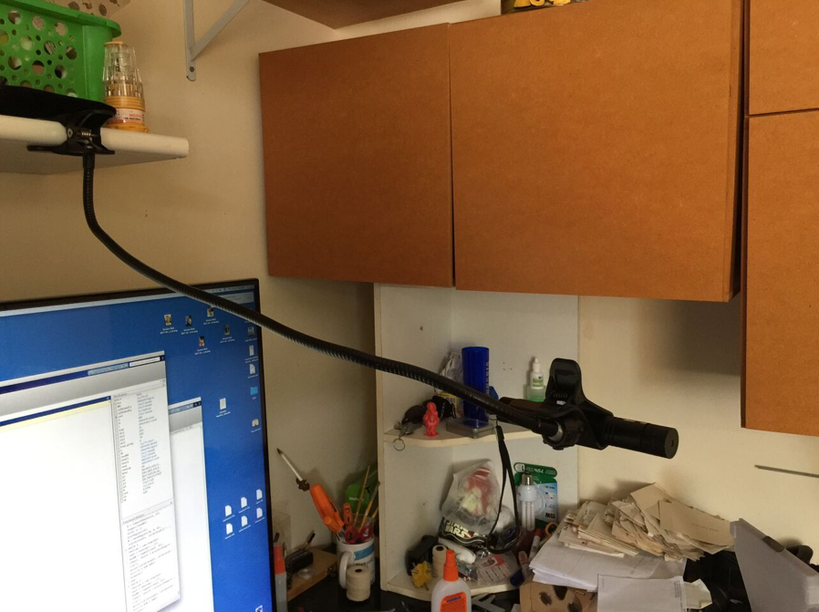
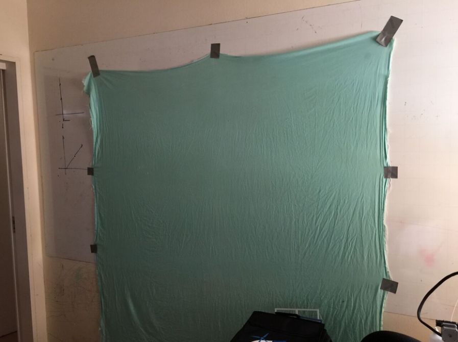
To finish this post, let me show you that you can even build your own wavefront sensor “mockup” at home! What I did in this experiment was to build a physical version of the Shack–Hartmann principle. The idea is to use a “blank wall” as detector and a webcam to record the light that arrives at the wall. This way I can simulate a giant set of detectors. Now the difficult part: the sub-aperure lenses… For this one, I had to make the cat jump. Instead of an array of hundreds of lenses in front of the “detector wall”, I uses a toy laser that comes with those diffraction crystals that projects “little star-like patterns” (see figure 7).
|
|
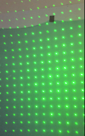
Figure 7: 1 – Toy laser (black stick) held in place. 2 – green “blank wall”. 3 – Diffraction pattern that generates a regular set of little dots.
With this setup, it was time to do some coding. Basically I did some Matlab functions to capture the webcam image of the wall with the dots. On those functions I setup some calibration computations to compensate for the shape and place of the dots on the wall (see video bellow). That calibration will tell me where the “neutral” atmosphere will project the points (centers of the sub apertures). Them, for each frame, I capture and process the image from the webcam. For each image, I compute the position of the processed centers with respect to the calibrated ones. With this procedure, I have, for each dot, a vector that points form the center to where it is. That is exactly the wavefront direction that the toy laser is emulating!
After that, it was a matter of having fun with the setup. I put all kinds of transparent materials in front of the laser and saw the “vector field” of the wavefront directions on screen. I even put my glasses and were able to see the same pattern the optical engineering saw when they were manufacturing the lenses! With a bit of effort I think I could even MEASURE (poorly of course) the level of astigmatism of my glasses!
The code is available in GitHub[2] but basically the loop consists in process each frame and show the vector field of the wavefront.
while 1
    newIcap = cam.snapshot();
    newI = newIcap(:,:,2);
    newBW = segment(newI, th);

    [newCx, newCy] = processImage(newBW, M, R);

    z = sqrt((calibratedCy-newCy).^2 + (calibratedCx-newCx).^2);
    zz = imresize(z,[480, 640]);

    figure(1);
    cla();
    hold('on');
    imagesc(zz(end:-1:1,:), 'alphadata',0.2)
    quiver(calibratedCy, calibratedCx, calibratedCy-newCy, calibratedCx-newCx,'linewidth',2);

    axis([1 640 1 480])

    drawnow()
end
Bellow you can watch the vídeo of the whole fun!
Conclusions
DIY projects are awesome for understanding theoretical concepts. In this case, the mix of simulation and practical implementation made very easy to understand how the device works. The use of the diffraction crystal in toy lasers is thought to be original, but I didn’t research a lot. If you know any experiment that uses this same principle, please let me know in the comments!
Again, thank you for reading until here! Feel free to comment o share this post. If you are an optical engineer, please correct me at any mistake I might have made on this post. It does not intend to teach about optics, but rather to share my passion for this subject that I know so little!
Thank you for reading this post. I hope you liked it and, as always, feel free to comment, give me feedback, or share if you want! See you in the next post!
References
[1] – Shack–Hartmann wavefront sensor
[2] – Matlab code
Hello,
Thank you so much for sharing your work online. I would like to measure the cylinder and spherical power in my glasses, and from what I read so far, I have to convert the wavefront to Zernike polynomials.
Could you point me in the right direction on how I can do this using your matlab code?
Thank you so much!
Hello there. Thank you for the comment.
The “conversion” from WFS slopes to Zernike polynomials consists in a simple projection. In the Matlab code I provide I don’t have a function for this projection because I always work on the command space (not the WFS slope space).
However, you can try this procedure:
1 – Generate the Zernike image corresponding to the mode you want to measure (comma, astigmatism, defocus, etc…) with the same size as you have your slopes measured (say 16×16)
2 – Normalise the image amplitude (so that its integral/sum) goes to 1 (be careful with the pixels outside the circular region).
3 – Compute the gradient of that image (gradient function on Matlab). This will give you the slopes of a pure Zernike mode.
4 – Multiply point to point your slope with those ones and add it up. This corresponds to performing an inner product between those.
5 – That is, more or less, the amount of that mode you have on your measurement.
Please notice that for small measurements, the set of discrete Zernike generated by this procedure are *NOT* orthogonal, so you will have just an approximation of the mode you want to measure. In practice, opticians use a WFS measurement with a lot of pixels to have a more precise projection.